Arleen A. Hill and Susan L. Cutter

Even with improvements in detection and warning systems, the direct losses associated with hazard events has steadily risen during the past three decades (van der Wink et al. 1998). Why is it that some places appear to be more disaster-prone whereas other communities seem to be somewhat immune from the impact of natural hazards? What makes some places more vulnerable to natural hazards than others? Is it that some communities are simply more at risk, or they have more people who lack adequate response mechanisms when the disaster strikes, or is it some combination of the two? This chapter reviews some of the contemporary hazard assessment tools and techniques that help us to understand societal vulnerability to hazards.

In its simplest form, vulnerability is the potential for loss. Like the term sustainability, vulnerability means different things to different people. For example, in the summary volume of this series, Mileti (1999) offered that vulnerability is “the measure of the capacity to weather, resist, or recover from the impacts of a hazard in the long term as

well as the short term” (p. 106). Vulnerability has been variously defined as the threat of exposure, the capacity to suffer harm, and the degree to which different social groups are at risk (Cutter 1996a). All are consistent with the more general definitions provided here. Perhaps equally important is the notion that vulnerability varies by location (or space) and over time—it has both temporal and spatial dimensions. This means that vulnerability can be examined from the community level to the global level, can be compared from place to place, and can be studied from the past to the present and from the present to the future. Most important to remember is that geography matters when discussing the vulnerability of people and places to environmental hazards.

There are many types of vulnerability of interest to the hazards community, but three are the most important: individual, social, and biophysical. Individual vulnerability is the susceptibility of a person or structure to potential harm from hazards. Scientists and practitioners from engineering, natural sciences, and the health sciences are primarily interested in this type of vulnerability. The structural integrity of a building or dwelling unit and its likelihood of potential damage or failure from seismic activity are examples of vulnerability at the individual-level scale. Building codes, for example, are designed to reduce individual structural vulnerability. Another example comes from the health sciences and focuses on the vulnerability of individual people, the potential exposure of the elderly to heat stress during the summer. In both instances, the characteristics of the individual structure (building materials, design) or person (age, diet, smoking habits, living arrangements) largely dictate their degree of vulnerability. The primary unit of analysis is an individual person, structure, or object.

On a more general level, we have social vulnerability, which describes the demographic characteristics of social groups that make them more or less susceptible to the adverse impacts of hazards. Social vulnerability suggests that people have created their own vulnerability, largely through their own decisions and actions. The increased potential for loss and a reduction in the ability to recover are most often functions of a range of social, economic, historic, and political processes that impinge on a social group’s ability to cope with contemporary hazard events and disasters. Many social scientists working in the field today, especially those working with slow-onset hazards (drought, famine, hunger) or those

working in developing world contexts, use the social vulnerability perspective. Some key social and demographic characteristics influencing social vulnerability include socioeconomic status, age, experience, gender, race/ethnicity, wealth, recent immigrants, tourists and transients (Heinz Center 2000a).

Biophysical vulnerability, the last major type, examines the distribution of hazardous conditions arising from a variety of initiating events such as natural hazards (hurricanes, tornadoes), chemical contaminants, or industrial accidents. In many respects, biophysical vulnerability is synonymous with physical exposure. The environmental science community mostly addresses issues of biophysical vulnerability based on the following characteristics of the hazards or initiating events: magnitude, duration, frequency, impact, rapidity of onset, and proximity. These types of studies normally would produce statistical accountings (or in some instances maps) that delineate the probability of exposure—that is, areas that are more vulnerable than others such as 100-year floodplains, seismic zones, or potential contamination zones based on toxic releases.

The integration of the biophysical and social vulnerability perspectives produces the “hazards of place” model of vulnerability (Cutter 1996a, Cutter et al. 2000). In our view, understanding the social vulnerability of places is just as essential as knowing about the biophysical exposure. The integrating mechanism is, of course, place. These places (with clearly defined geographic boundaries) can range from census divisions (blocks, census tracts), to neighborhoods, communities, counties, states, regions, or nations. Among the many advantages of this approach is that it permits us to map vulnerability and compare the relative levels of vulnerability from one place to another or from region to region and, of course, over time. In this way, we have a very good method for differentiating disaster-prone from disaster-resilient communities, identifying what suite of factors seem to influence the relative vulnerability of one place over another, and monitoring how the vulnerability of places changes over time as we undertake mitigation activities.

As mentioned in Chapter 1, the terms risk and hazard have slightly different meanings. It should come as no surprise that, in developing risk or hazards assessments, there are subtle differences in meaning and approaches as well. Risk assessment, is a systematic characterization of the probability of an adverse event and the nature and severity of that event

(Presidential/Congressional Commission on Risk Assessment and Risk Management 1997). Risk assessments are most often used to determine the human health or ecological impacts of specific chemical substances, microorganisms, radiation, or natural events. Risk assessments (the relationship between an exposure and a health outcome) normally focus on one type of risk (e.g., cancers, birth defects) posed by one substance (e.g., benzene, dioxin) in a single media (air, water, or land). In the natural-hazards field, risk assessment has a broader meaning, and involves a systematic process of defining the probability of an adverse event (e.g., flood) and where that event is most likely to occur. Much of the scientific work on modeling, estimating, and forecasting floods, earthquakes, hurricanes, tsunamis, and so on, are examples of risk assessments applied to natural hazards (Petak and Atkisson 1982).

Vulnerability assessments include risk/hazard information, but also detail the potential population at risk, the number of structures that might be impacted, or the lifelines, such as bridges or power lines (Platt 1995), that might be damaged. Vulnerability assessments describe the potential exposure of people and the built environment. The concept of vulnerability incorporates the notion of differential susceptibility and differential impacts. Exposures may not be uniformly distributed in space, nor is the societal capacity to recover quickly the same in all segments of the population. It is the exposure to hazards and the capacity to recover from them that define vulnerability. Thus, vulnerability assessments must incorporate both risk factors and social factors in trying to understand what makes certain places or communities more susceptible to harm from hazards than others. This makes vulnerability assessments more difficult to undertake than simple risk analyses because they require more data (some of which may not be available) and have more complex interactions that need careful consideration.

For our purposes, however, we use the terms risk assessment and hazards assessment interchangeably. There is a rich literature on risk/ hazards assessments and vulnerability assessments that range from very localized experiences to the development of global models of vulnerability (Ingleton 1999). We describe a number of these approaches in the following section.

There have been many notable advances in hazards and risk modeling during the past two decades. These are described in more detail in the

following subsections.

The majority of risk estimation models are hazard specific. Some are designed for very general applications, such as the hurricane strike predictions issued by the National Hurricane Center (NHC), whereas others are designed to aid in the selection of specific protective actions based on the plume from an airborne chemical release. It is impossible to adequately review all of the existing risk estimation models. Instead, we highlight a number of the most important and widely used within the hazards field. A more detailed description of these models can be found in Appendix A.

Dispersion models estimate the downwind concentrations of air pollutants or contaminants through a series of mathematical equations that characterize the atmosphere. Dispersion is calculated as a function of source characteristics (e.g., stack height, rate of pollution emissions, gas temperature), receptor characteristics (e.g., location, height above the ground), and local meteorology (e.g., wind direction and speed, ambient temperature). Dispersion models only capture the role of the atmosphere in the delivery of pollutants or an estimation of the potential risk of exposure. They do not provide an estimate of the impacts of that exposure on the community or individuals because those specific environmental and individual factors are not included in the model. They are crude representations of airborne transport of hazardous materials and lead to over- or underestimation of concentrations (Committee on Risk Assessment of Hazardous Air Pollutants 1994).

Many of the dispersion models currently in use, such as the U.S. Environmental Protection Agency’s (USEPA) Industrial Source Complex (ISC), can accommodate multiple sources and multiple receptors. Another aspect of these models is the ability to include short-term and longterm versions, which can model different timing and duration of releases (USEPA 1995). Regulators, industries, and consultants commonly use ISCST3, the short-term version. In addition to permitting and regulatory evaluations, dispersion models have been applied to studies of cancer risk from urban pollution sources (Summerhays 1991). At a National Priority List landfill in Tacoma, Washington, the ISCST3 model was used

to predict the maximum ground-level concentrations of volatile organic compounds vented from the contaminated site (Griffin and Rutherford 1994).

The most important air dispersion model for emergency management is the Areal Locations of Hazardous Atmospheres (ALOHA)/ Computer-Aided Management of Emergency Operations (CAMEO) model of airborne toxic releases, developed by the USEPA. The ALOHA model uses a standardized chemical property library as well as input from the user to model how an airborne release will disperse in the atmosphere after an accidental chemical release (USEPA 2000a). Currently, the model is used as a tool for response, planning, and training by government and industry alike. Graphical output in the form of a footprint with concentrations above a user-defined threshold can be mapped (Figure 2-1) using a companion application (MARPLOT). CAMEO is a system of software applications used to plan for and respond to chemical

FIGURE 2-1 Stylized version of the computer output from the ALOHA model, showing the plume path from an airborne toxic release. See USEPA 2000b, http://response.restoration.noaa.gov/cameo/aloha.html for other examples.

emergencies. Developed by the USEPA’s Chemical Emergency Preparedness and Prevention Office (CEPPO) and the National Oceanic and Atmospheric Administration (NOAA), it is designed to aid first-responders with accurate and timely information. Integrated modules store, manage, model, and display information critical to responders. CAMEO has a database of response recommendations for 4,000 chemicals and works with the ALOHA air dispersion model and MARPLOT mapping module to provide firefighting, physical property, health hazard, and response recommendations based on the specific chemical identified (USEPA 2000b).

Potential storm surge inundation of coastal areas is determined by the Sea, Lake, and Overland Surges (SLOSH) model developed by the U.S. National Weather Service (NWS) in 1984 (Jelesnianski et al. 1992). As a two-dimensional, dynamic, numerical model, SLOSH was developed initially to forecast real-time hurricane storm surges. SLOSH effectively computes storm surge heights, where model output is a maximum value for each grid cell for a given storm category, forward velocity, and landfall direction. SLOSH is used primarily in pre-impact planning to delineate potential storm surge inundation zones and can be repeated for different hurricane scenarios at the same location (Garcia et al. 1990).

NOAA recommends that emergency managers use two slightly different model outputs in their evacuation planning—MEOW and MOM. MEOW is the Maximum Envelope of Water and represents a composite of maximum high-water values per grid cell in the model run. The National Hurricane Center (NHC) combines the values for each grid cell and then generates a composite value for a specific storm category, forward velocity, and landfall direction. Of more use to emergency managers is the MOM (Maximum of the MEOW), a composite measure that is the maximum of the maximum values for a particular storm category (NOAA 2000a). In other words, this is the worst-case scenario. SLOSH model output is in the form of digital maps that show the calculated storm surge levels as a series of contours or shaded areas (Figure 2-2, see color plate following page 22). These maps form the basis for local risk estimates upon which evacuation plans are developed. Comparisons of the SLOSH real-time forecasts and actual observations of storm surge confirm that this model is extremely useful to emergency management officials at local, state, and national levels. This output provides not only

an important pre-impact planning tool (locating shelters and evacuation routes), but also contributes to recovery and mitigation efforts in coastal communities (Houston et al. 1999). The model also has been utilized in the revision of coastal flood insurance rate maps (FIRMS).

Regional SLOSH model coverage includes the entire Gulf and Atlantic coastlines of the United States and parts of Hawaii, Guam, Puerto Rico, and the Virgin Islands. Modeling of SLOSH basins has been extended internationally to include the coastal reaches of the People’s Republic of China and India (NOAA 2000a).

Both long-range and storm-specific forecasting and modeling efforts exist for hurricanes. The NHC provides forecast information on storm track, storm intensity, and surface winds for individual storms. The long-or extended-range forecasts categorize or predict the activity of a specific basin over a specific season. Predictions or estimations for the Atlantic Basin are based on statistical models and the experience of a forecasting team. The statistical model incorporates global and regional predictors known to be related to the Atlantic Basin hurricane season, mostly derived from historical data. The model is run and then qualitatively adjusted by the forecast team based on supplemental information not yet built into the model (Gray et al. 1999).

Advances in weather satellites, forecasting models, research, and empirical data have led to a reduction of errors in forecasted path by 14 percent in the past 30 years (Kerr 1990). Although some of the statistical models are being phased out, the more dynamic models taking their place, such as GFDL, UKMET, and NOGAPS (see Appendix A), allow the NHC to develop an average of these storm-track predictions and then send appropriate warning messages. Although this approach has led to a decrease in errors in strike probabilities (180 miles error at 48 hours out; 100 miles error at 24 hours out) it has resulted in an increase in the amount of coastline that must be warned per storm (Pielke 1999). There are a number of explanations for this: (1) the desire to base evacuation decisions on the precautionary principle and develop a very conservative estimate of landfall based on official NHC forecasts; (2) the westward or left bias of many of the models, thus the need to warn a larger area to avoid any last-minute change in the track; and (3) larger coastal populations requiring longer evacuation times.

At the same time, improvements in cyclone intensity modeling (SHIFOR, SHIPS, CLIPER; see Appendix A) allow forecasters to improve their estimation of the intensity of these systems by 5-20 knots. This type of modeling provides better estimates of wind fields at the surface and near surface. With improved air reconnaissance and the use of Global Positioning System drop-windsondes (Beardsley 2000), we now have a better understanding of wind patterns not only at the surface but throughout the entire storm system. Additional information on hurricane forecasting models can be found in Appendix A and at NOAA’s Web site (NOAA 2000a).

The issuance and communication of tornado watches and warnings is a vital part of protecting lives and property from severe storms. A complex network that relies on both sophisticated equipment and trained observers monitors the development of severe storm cells. NOAA’s National Severe Storms Forecast Center (NSSFC) in Kansas City, Missouri, the NWS SKYWARN System, radar and trained spotters, and the NOAA National Severe Storms Laboratory (NSSL) in Norman, Oklahoma are part of the complex network.

In partnership with the NWS, the NSSL generates forecasts based on numerical weather prediction models (see Appendix A). These models provide temperature, pressure, moisture, rainfall, and wind estimates as well as geographically tracking severe storms and individual storm cells.

Doppler radar provides estimates of air velocity in and near a storm and allows identification of areas of rotation. Detection of potentially strong thunderstorm cells (also called mesocyclone signatures) can be identified in parent storms as much as 30 minutes before tornado formation. Signatures of the actual tornadic vortex can also be observed on Doppler radar by the now-distinct hook-shaped radar echo (Figure 2-3, see color plate following page 22). The signature detection process remains subjective, however, and thus prone to human errors in image interpretation, especially in real time. Some tornado-generating storms have typical signatures, but others do not. Also, some storms with these mesocyclone signatures never generate tornadoes. Nevertheless, Doppler radar has helped increase the average lead time for risk estimation and the implementation of tornado warnings from less than 5 minutes in the late 1980s to close to 10 minutes today (Anonymous 1997).

Estimating flood risk depends on the type of flooding: coastal (storm surge and tsunamis), riverine (river overflow, ice-jam, dam-break), and flash floods (with many different subcategories) (IFMRC 1994). Coastal flooding risk due to storm surge (see storm surge discussion p. 19) is developed by a slightly different set of models than riverine or flash floods. The complex relationship between hydrological parameters such as stream channel width, river discharge, channel depth, topography, and hydrometeorological indicators of intensity and duration of rainfall and runoff produces estimates of the spatial and temporal risk of flooding.

Working in tandem, the U.S. Geological Survey (USGS) and the NWS provide relevant risk data for flood events. The NWS has the primary responsibility for the issuance of river forecasts and flood warnings through its 13 Regional River Forecast Centers. The USGS provides data on river depth and flow through its stream gauge program, resulting in real-time river forecasting capability. In fact, real-time river flow data for gauged streams are now available on the World Wide Web for anyone to use (USGS 2000a). Flow or discharge data are more difficult to measure accurately and continuously, and so, hydrologists employ rating curves, which are pre-established river stage/discharge relations that are periodically verified by field personnel.

NOAA’s Hydrometeorological Prediction Center (HPC) is another important partner in determining flood risk. The HPC provides medium-range (3-7 days) precipitation forecasts as well as excessive rainfall and snowfall estimates. Through the use of quantitative precipitation forecasts, forecasters can estimate expected rainfall in a given basin and the accumulated precipitation for 6-hour intervals. This information is transmitted to the NWS River Forecast Centers and is also available in real time (HPC 2000). Using river stage, discharge, and rainfall, hydrologic models are employed to see how rivers and streams respond to rainfall and snowmelt. These modeled outputs provide the risk information that is transmitted to the public—height of the flood crest, date and time that river is expected to overflow its banks, and date and time that the river flow is expected to recede within its banks (Mason and Weiger 1995).

The Coastal Vulnerability Index evaluates shoreline segments on their risk potential from coastal erosion or inundation (Gornitz et al.

1994, FEMA 1997a). High-risk coastlines are defined by low coastal elevations, histories of shoreline retreat, high wave/tidal energies, erodible substrates, subsidence experience, and high probabilities of hurricane and/or tropical storm hits. The index uses 13 biophysical variables such as elevation, wave heights, hurricane probability, and hurricane intensity, which are ranked from low to high (1 to 5). Three different indicators were developed (permanent inundation, episodic inundation, and erosion potential) from these 13 variables and then weighted to produce an overall score for each of the 4,557 U.S. shoreline segments examined. The data are geocoded and can be used in conjunction with other geographic information to produce vulnerability assessments.

A recent report completed by the Heinz Center (2000b) delineates the potential erosion hazard for selected study segments of U.S. coastlines from Maine to Texas, southern California to Washington, and along the Great Lakes. Using historic shoreline records dating back to the 1930s or earlier, historic rates of erosion are used to calculate an annual erosion rate. These rates of erosion are then mapped using the current shoreline as the base, with projections to 30 years and 60 years. The future rates of erosion are conservative estimates. For example, there is no consideration of accelerated sea-level rise due to increased global warming or increased development along the coastline, both of which might accelerate erosion rates.

Another approach to coastal risk examines the potential hazards of oil spills on coastal environments. The Environmental Sensitivity Index (ESI) is used to identify shoreline sensitivity to oil spills based on the nature of the biological communities, sediment characteristics, and shoreline characteristics (including both physical attributes and cultural resources) (Jensen et al. 1993, 1998). Using remote sensing to monitor changes in coastal wetland habitats and a geographic information system to catalog, classify, and map sensitive areas, the ESI has been applied not only to coastlines, but to tidal inlets, river reaches, and regional watersheds.

Seismic risks are delineated in two different ways—through the identification of specific known surface and subsurface faults and through the regional estimation of ground motion expressed as a percentage of the peak acceleration due to gravity. Both rely on historical seismicity, using the past as a key to future earthquake activity. Assessments that

yield maps of active faults or data on historical seismic activity are the simplest forms of seismic risk assessment. However, probabilistic maps that incorporate the likelihood of an event or exceedence of some ground-shaking threshold are now being generated and increasingly used as estimators of seismic risk.

Two approaches used in assessing an earthquake hazard are probabilistic and deterministic methods. The probabilistic approach attempts to describe the integrated effects from all possible faults at an individual site. These assessments recognize uncertainties in our knowledge of fault parameters, earthquake magnitude and intensity, and the responses of built structures. The probabilistic method requires the user to define the level of risk for consideration, thus introducing the concept of acceptable risk and the consideration of critical facilities (Yeats et al. 1997). Probabilistic studies can be further divided into time-dependent and time-independent models. Recent examples include the Working Group 2000 report on the San Francisco Bay Area (time-dependent) (USGS 2000b) and the national seismic hazard maps (time-independent) (Frankel et al. 1997, USGS 2000c).

Deterministic methods specify a magnitude or level of ground shaking to be considered. Often, a single fault is considered and seismic parameters for a “maximum credible” event are applied. The probability of that earthquake occurring is not incorporated in the analysis. Instead, three types of information are used: historical and instrumental record, evidence and physical parameters from seismogenic faults, and/or paleoseismic evidence of prehistoric earthquakes (Yeats et al. 1997). These types of models commonly represent a “worst-case scenario,” or the maximum risk people or a particular place could be exposed to.

USGS maps provide estimates of the probability of exceeding certain levels of ground motion in a specified time (e.g., 10 percent probability of exceedence in 50 years). Time periods range from 100 to 2,500 years (Algermissen and Perkins 1976, Algermissen et al. 1982). National seismic hazard maps have recently been generated (Frankel et al. 1996) and have been used to develop county-level seismic risk assessments based on the default soil site conditions (Nishenko 1999, FEMA 2000a). These seismic maps are now used in the National Earthquake Hazards Reduction Program’s (NEHRP) guidance for hazards loss reduction in new and existing buildings.

The science of vulnerability assessments is not nearly as advanced as for risk estimation. In fact, vulnerability science is really in its infancy. Whether it is an analysis of the potential physical and economic impacts of climate change on climate-sensitive sectors such as agriculture, water resources, and the like (U.S. Country Studies Program 1999) or the integration of vulnerability into sustainable development programs (OAS 1991), the issue remains the same. What indicators do we use to measure vulnerability and how do we represent that information to decision makers?

More often than not, vulnerability indicators are single variables (lifelines, infrastructure to support basic needs, special-needs populations, schools), but occasionally multidimensional factors such as food aid, social relations, and political power have been incorporated (Blaikie et al. 1994). The research on vulnerability assessments is characterized by case studies ranging from very localized analyses of a city (Colten 1986, 1991), to a county or state (Liverman 1990), to more regional perspectives (Downing 1991, Lowry et al. 1995) and by a focus on a single hazard (Shinozuka et al. 1998). There are a variety of methods used to determine vulnerability, and many include some form of geographic information system (GIS) and maps that convey the results.

Activities within the Organization of American States (OAS) provide some of the most innovative examples of the role that hazard vulnerability plays in international development assistance. Through its Working Group on Vulnerability Assessment and Indexing, OAS is trying to develop a common set of metrics for measuring vulnerability to natural hazards that could then be used in disaster preparedness and response efforts and in financing disaster reduction among member nations. The most advanced efforts in assessing vulnerability are through the Caribbean Disaster Mitigation Project (OAS 2000).

Within the United States, hazard identification and risk assessment are among the five elements in FEMA’s (1995) National Mitigation Strategy. Project Impact has called for the undertaking of hazard identification (risk assessment) and vulnerability assessment, yet it provides very little technical guidance on how to conduct such analyses other than consulting with FEMA or developing partnerships with professional associations. Despite this lack of direction, a number of states have adopted innovative tools for vulnerability assessments. For example, Florida utilized a commercial product, the Total Arbiter of Storms (TAOS) model,

developed by Watson Technical Consulting (2000) (and distributed through Globalytics). This model simulates the effect of selected hazards (waves, wind, storm surge, coastal erosion, and flooding) as well as their impact on both physical and built environments including damage and economic loss estimates. Aspects of the model can also be used for real-time hurricane tracking, track forecasting, and probabilistic modeling of hurricane and tropical cyclone hazards. The TAOS hazard model has also been used by a number of Caribbean nations to assess the risk of storm surge, high wind, and wave hazards and their local impact (OAS 2000). Florida has also developed a manual for local communities, which uses a GIS-based approach to risk mapping and hazards assessment, including specific guidance on hazard identification and vulnerability assessment (State of Florida 2000).

There are a number of noteworthy efforts to determine vulnerability using single hazards. The most advanced are the U.S. Agency for International Development’s (U.S. AID) Famine Early Warning System (FEWS) and the United Nations Food and Agricultural Organization’s Africa Real Time Environmental Monitoring Information System (ARTEMIS) (Hutchinson 1998). Both of these monitoring programs, which include remote sensing and GIS, are part of the Global Information and Early Warning System (GIEWS) and provide data for vulnerability assessments that evaluate national and international food security issues. The vulnerability assessment is used to describe the nature of the problem and classifies, both qualitatively and quantitatively, who is affected, the impacted area, and potential interventions. These assessments are done at a variety of levels from the household to the national level. Finally, a food security and vulnerability profile can be generated that gives a historic analysis of food availability and access. This profile also provides a more comprehensive view of the level, trends, and factors that influence food security (or insecurity) for individual population groups or nations. These profiles can also be mapped to illustrate their vulnerability geographically (Figure 2-4).

Another example of a hazard-specific vulnerability assessment was conducted by NOAA’s Coastal Services Center for hurricane-induced coastal hazards in Alabama (NOAA Coastal Services Center NDa). In addition to that product, they have also produced a GIS-based assessment tool that defines risk areas, identifies critical infrastructure, and

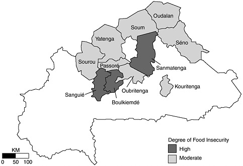
FIGURE 2-4 Food insecurity in Burkina Faso (1999-2000) based on U.S. AID’s FEWS current vulnerability assessment for March 2000. Source: http://www.fews.org/va/vapub.html.

maps the potential impact from coastal hazards. Using a case study of coastal hazards in New Hanover County, North Carolina, the tool provides a tutorial on how to conduct vulnerability assessments and develop priorities for hazard mitigation opportunities (NOAA Coastal Services Center NDb).

A number of multihazard vulnerability assessments have been conducted, but all are quite localized in scale. For example, Preuss and Hebenstreit (1991) developed a vulnerability assessment for Grays Harbor, Washington. Risk factors included primary and secondary impacts from an earthquake, including a tsunami event and toxic materials release. Social indicators included land use and population density and distribution. Another example is the county-level work by Toppozada et al. (1995) on Humboldt and Del Norte, California. Mapping the risk information (tsunami waves, ground failure, fault rupture, liquefaction, and landslides) and societal impacts (buildings, infrastructure, lifelines) allowed for the delineation of vulnerable areas within the counties. The

work by the USGS on Hurricane Mitch and its devastating impact in Central America is another example (USGS 1999).

Lastly, the work of Cutter and colleagues (Mitchell et al. 1997, Cutter et al. 2000) in Georgetown County, South Carolina, provides one of the most comprehensive methodologies for county-level vulnerability assessments. Utilizing both biophysical risk indicators (e.g., hurricanes, seismicity, flooding, hazardous materials spills) and social vulnerability indicators (population density, mobile homes, population over 65, race) within a GIS allows for determining the geographic distribution of vulnerability within the county. Biophysical risk was determined by the historic frequency of occurrence of hazard events in the county and applied to the specific impacted areas (e.g. 100-year floodplain for flood occurrence; SLOSH-model inundation zones for hurricanes). Areas of high social vulnerability can be examined independently of those areas of high biophysical risk. They can also be examined together to get an overall perspective of the total vulnerability of the country to environmental hazards. More importantly, this methodology enables the user to examine what specific factors are most influential in producing the overall vulnerability within the county.

Loss estimates are important in both pre-impact planning and in post-disaster response, yet we have very little systematic data on what natural hazards cost this nation on a yearly basis. In addition, there is no standardized estimation technique for compiling loss data from individual events, or any archiving system so that we can track historic trends (NRC 1999a, b). Although we are improving our data collection on biophysical processes (risk and vulnerability), some have argued that our data on natural hazard losses resembles a piece of Swiss cheese—a database with lots of holes in it.

There are many different types of loss estimation techniques that are available. Their use largely depends on what types of losses one is interested in measuring (economic, environmental) and the scale (individual structures or entire county or nation) of estimation.

FEMA, in partnership with the National Institute for Building Sciences (NIBS), developed HAZUS (Hazards US). This is a tool that can be

used by state and local officials to forecast damage estimates and economic impacts of natural hazards in the United States. At present, HAZUS includes the capability to use both deterministic and probabilistic earthquake information for loss estimation. Although the earthquake loss estimation module is the only one available at the moment, HAZUS eventually will include a wind-loss component and a flood-loss module (scheduled for release in 2002/2003).

In HAZUS, local geology, building stock and structural performance, probabilistic scenario earthquakes, and economic data are used to derive estimates of potential losses from a seismic event. A modified GIS displays and maps the resulting estimates of ground acceleration, building damage, and demographic information at a scale determined by the user (e.g., census tract, county). Designed for emergency managers, planners, city officials, and utility managers, the tool provides a standardized loss estimate for a variety of geographic units. Generally speaking, four classes of information are provided: (1) map-based analyses (e.g., potential ground-shaking intensity), (2) quantitative estimates of losses (e.g., direct recovery costs, casualties, people rendered homeless), (3) functional losses (e.g. restoration times for critical facilities), and (4) extent of induced hazards (e.g., distribution of fires, floods, location of hazardous materials). HAZUS calculates a probable maximum loss. It also calculates average annual loss, a long-term average that includes the effects of frequent small events and infrequent larger events (FEMA 2000a).

At present, losses are generated on the basis of “scenario earthquakes,” which is a limitation of the tool because the location and magnitude of the “scenario earthquakes” may not represent the actual magnitude or location of future events. Default data describe geology, building inventory, and economic structure in general terms and can be used to produce very generalized loss estimates on a regional scale. However, communities must supplement these general data with local-level data in order to assess losses for individual communities such as cities, towns, and villages. Unfortunately, these local-level data often are unavailable. Despite these limitations, HAZUS does enable local communities to undertake a “back of the envelope” quick determination of potential losses from a pre-designed seismic event. HAZUS also allows users to do rapid post-event assessments. The software was tested in September 2000 with the Labor Day earthquake in Yountville, California. The damage estimates predicted by HAZUS for an earthquake of the same size and magnitude as Yountville turned out to be very similar to the actual level of destruction and damage.

To be more useful at the local level for planning and mitigation activities, however, the default inventory of structures and infrastructure must be updated at the local level. Improvements in local risk factors (geology) are also required inputs for more detailed analyses at the local level. As is the case with many models, there are acknowledged limitations (FEMA 1997c). Among the cautions are:

• Accuracy of estimates is greater when applied to a class of buildings than when applied to specific buildings.

• The accuracy of estimated losses associated with lifelines is less accurate than those associated with the general building stock.

• There is a potential overestimation of losses, especially those located closed to the epicenter in the eastern United States due to conservative estimates of ground motion.

• The extent of landslide potential and damage has not been adequately tested.

• The indirect economic loss module is experimental and requires additional testing and calibration.

• There is uncertainty in the data and a lack of appropriate metadata (or sources) for many of the components.

• There is spatial error due to the reconciliation of physical models (e.g., ground shaking) with census-tract demographic data.

The insurance industry has a long tradition of involvement in exposure assessment and risk management. Many of these tools and techniques are described in more detail elsewhere (Kunreuther and Roth 1998).

In most instances, financial risk assessment is based on probabilistic models of frequency and magnitude of events. In addition, proprietary data on insured properties, including the characteristics of those holdings are available and subsequently used to develop applications of expected to worst-case scenarios. For example, the Insurance Research Council (IRC) (IIPLR and IRC 1995) released a report on the financial exposure of states, based on the Hurricane Andrew experience. They found, along with increased population in the coastal area, that there is a significant rise in the value of insured properties, resulting in a potential loss of more than $3 trillion in 1993. This has increased since then.

Other examples of financial risk models that are used include Applied Insurance Research’s catastrophe model and Risk Management

Solutions’ Insurance and Investment Risk Assessment System (Heinz Center 2000a). To protect themselves from catastrophic losses, insurance companies utilize the reinsurance market as a hedge against future losses from natural hazards. Reinsurers use very sophisticated risk assessment models to calculate the premiums they charge to the insurance company and rely quite extensively on the scientific community (Malmquist and Murnane 1999). Reinsurers need to know the worstcase scenario (or probable maximum loss) and incorporate the following data in their calculations: hazard risk (intensity, frequency, and location), location of insured properties (homes, businesses, cars, etc.), existing insurance, and insurance conditions (deductibles, extent of coverage). Examples include PartnerRe’s tropical cyclone model (Aller 1999) and Impact Forecasting’s natural hazard loss estimation model for earthquakes and hurricanes (Schneider et al. 1999). The latter is especially interesting because it includes a mitigation application.

Most of the hazard loss estimation tools and techniques focus on the built environment such as buildings, transportation networks, and so forth. The loss of ecological systems and biodiversity is also important when thinking about vulnerability. These natural resources are the building blocks of modern economic systems. While there are many causes of ecological loss, most of them derive from human activities—urban encroachment, land-use changes, deforestation, introduction of foreign species, environmental degradation, and natural disasters. Historically, biodiversity loss was handled via individual species protection (endangered and threatened species) or through habitat conservation (mostly through national parks, wilderness areas, or biosphere reserves) (Cutter and Renwick 1999). One technique for the identification of these critical habitats and the species that live there is gap analysis, a program run by the National Biological Survey. Using remote-sensing and GIS techniques, gap analysis maps land cover, land ownership patterns, vegetation types, and wildlife to identify areas that are underrepresented in protected management systems, hence the name “gap” analysis (LaRoe et al. 1995, Jensen 2000). Gap analysis has been successfully used in locations throughout the nation to reduce ecological losses.

Another approach to ecological risk assessment is to examine the potential impact that human activities have on individual plants and animals or on ecosystems. Ecological risk is defined as the potential harm

to an individual species or ecosystem due to contamination by hazardous substances including radiation. Ecological risk assessments (ERAs) provide a quantitative estimate of species or ecosystems damage due to this contamination by toxic chemicals. ERAs are similar in nature and scope to human health risk assessments, although the targeted species is different. The USEPA provides a set of guidelines for conducting ERAs, which have focused on single species, and single contaminants (USEPA 2000c). However, the science of ERAs is quickly evolving to include multiple scales, stressors (contaminants), and endpoints in order to achieve more robust and holistic risk assessments of threatened ecosystems, but it is not quite there yet (Suter 2000).

Thus far, we have examined methods that help to estimate risk, assess vulnerability, and estimate financial and ecological losses from a single phenomenon. There are, however, techniques especially designed to provide a comparison among places with respect to risk levels and vulnerability, and these are described below.

In 1987, the USEPA released a report, Unfinished Business (USEPA 1987), which set the stage for a realignment of agency priorities. There was a fundamental change at the agency—a movement away from pollution control to pollution prevention and risk reduction. To more effectively utilize resources and prioritize and target the most severe environmental problems, the USEPA developed the CRA tool (Davies 1996). Although many argue that the results of the ranking exercise are sensitive to the specific procedures used including categorization (Morgan et al. 2000), CRA does allow the incorporation of technical expertise, stakeholders, and policy makers in targeting activities and prioritizing risks and resources to reduce them. A number of case studies have been completed with varying degrees of success, the most important one being the tendency of the process to build consensus among the participants on the prioritizing of environmental problems (USEPA 2000d).

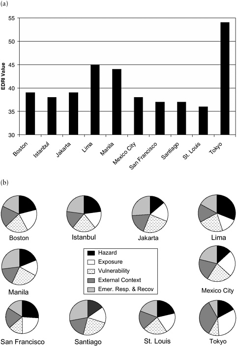
As part of the International Decade for Natural Disaster Reduction (IDNDR 1990-2000), the United Nations established an urban seismic risk initiative. The Risk Assessment Tools for Diagnosis of Urban Areas Against Seismic Disasters (RADIUS) developed practical tools for seismic risk reduction in nine case-study cities, especially in the developing world (Okazaki 1999). In addition to an assessment of seismic risk (exposure) and vulnerability, an action plan for preparedness against future earthquake disasters is also required. Based on input data (population, building types, ground types, and lifelines), and a hypothetical scenario earthquake such as the Hanshin-Awaji earthquake in Kobe, Japan, the output indicators include seismic intensity (Modified Mercalli Scale), building damage estimates, lifeline damage, and casualties. In addition to the nine detailed case studies, 103 other cities are carrying out seismic risk assessments based on this methodology (Geohazards International 2000). On a more general level, urban seismic risks can be compared using the Earthquake Disaster Risk Index (EDRI) (Cardona et al. 1999). The EDRI compares urban areas for the magnitude and nature of their seismic risk according to five factors: hazard, vulnerability, exposure, external context, and emergency response and recovery. Urban areas can be compared using any or all of these dimensions (Figures 2-5a and 2-5b).

The United Nations Disaster Relief Organization produced an assessment of natural hazard vulnerability at the beginning of the IDNDR in 1990. Using a 20-year history of natural hazards and their financial impact on individual nations (expressed as a percentage of GNP), the Disaster-Proneness Index provides a preliminary evaluation of the relative hazardousness of nations (UNEP 1993). Island nations, especially those in the Caribbean, rank among the top 10 on this index, as do a number of Central American (El Salvador, Nicaragua, Honduras), African (Ethiopia, Burkina Faso, Mauritania), and Asian (Bangladesh) countries. When mapped, the most disaster-prone countries are in the developing world. This is not surprising, given their biophysical and social vulnerability and the inability to respond effectively in the aftermath of the event or to mitigate future disasters (Cutter 1996b). There has been no subsequent update or revision of this original index.

A newly emerging vulnerability index uses the concept of sustainability in understanding vulnerability to hazards. In January 2000, the World Economic Forum, the Yale Center for Environmental Law and Policy, and the Center for International Earth Science Information Network released the Pilot Environmental Sustainability Index. This prototype was designed to measure sustainability of national economies using one composite measure with five components: environmental systems (healthy land, water, air, and biodiversity), environmental stresses and risks, human vulnerability to environmental impacts, social and institutional capacity to respond to environmental challenges, and global stewardship (international cooperation, management of global commons). While still in its developmental stage, the Pilot Environmental Sustainability Index shows much promise in differentiating countries that are achieving environmental sustainability or are ranked in the top quintile (New Zealand or Canada) from those that rank in the lowest quintile (Mexico, India) (World Economic Forum 2000).

This chapter examined the range and diversity of current methods used to assess environmental risks and hazards and societal vulnerability to them. Some approaches are hazard specific whereas others incorporate multiple hazards. Global comparisons of risks and hazards exist, yet most of the assessment techniques and their applications are hazard specific or geographically restricted. In some instances the state-of-the-art science and technology have not made their way into practice, whereas in other cases the needs of the emergency management community are driving the development of new and innovative approaches to measuring, monitoring, and mapping hazard vulnerability.

Our review of the contemporary hazard and vulnerability methods and models did not include two important considerations that will drive the next generation of models and methodologies. First, we did not provide an explicit discussion of the underlying and contextual factors that increase the vulnerability of people and places: urbanization, demographic shifts, increasing wealth, increasing poverty, labor markets, cultural norms and practices, politics, business, and economics. Changes in any of these contextual factors will either amplify or attenuate vulner-

ability in the future or result in greater regional variability in hazardousness.

Second, we did not address the issue of how current hazards and risk assessment methods and practices might actually contribute to the relocation of risk and vulnerability (either geographically or into the future). This transfer of risk and vulnerability (variously called risk relocation or risk transference) (Etkin 1999) in either time (present to future) or space (one region or area to another) is an important consideration in assessing hazards and vulnerability. Yet our current methods and models are woefully inadequate in this regard, especially in determining some of the ethical and equity questions involved in the transference itself.

The implementation of public policies based on our hazards assessments have the potential to reduce vulnerability in the short term (a sea wall to protect against coastal erosion) yet they may ultimately increase vulnerability in the longer term, thus affecting the next generation of residents. Understanding, measuring, and modeling future risk and vulnerability are among the many environmental challenges we will face in the coming decade. The next chapter examines another future challenge—how to visually represent hazards and risks in ways that are both scientifically meaningful and understandable to a general audience.