CHAPTER 4
Results of the Analytical Program

4.1 Sectional Analysis

An in-depth sectional analysis was conducted to validate the flexural behavior and deformability of prestressed beams and girders with SS strands. This analysis covered four topics: (1) pretensioned beams, (2) posttensioned beams, (3) prestressed concrete piles, and (4) the shear behavior of prestressed beams, which are discussed in Appendix C. An analytical model based on the layer method and strain compatibility approach was developed to assess the flexural behavior of the girders. An AASHTO Type I girder was selected for this analysis to validate the experimental results.

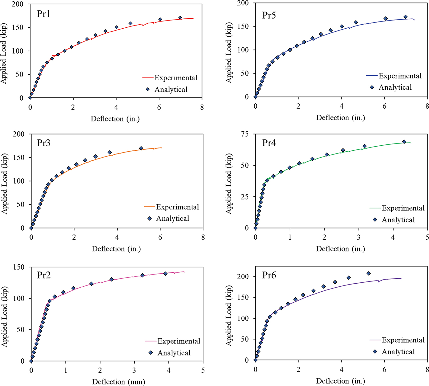
Comparison of the load-deflection curves generated by the model with experimental data for all tested girders demonstrated strong agreement, confirming the accuracy of the analytical approach. The results are presented in Figure 37.

Unlike the CS strand, rupture of SS strands is a failure mode that must be considered in addition to the concrete crushing failure mode. When the failure mode is rupture of SS strands, the concrete strain at the top fiber of the member is less than the ultimate value specified in LRFD BDS (2024), so the stress block factors α₁ and β₁ provided in the LRFD BDS should not be used because the underlying assumptions for use of the stress block are not met.

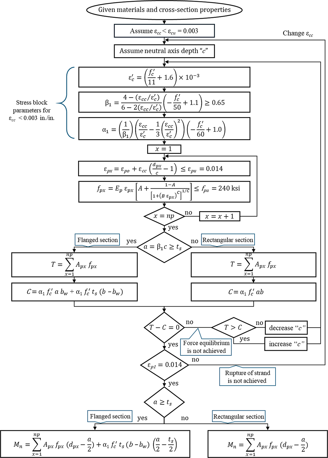
Belarbi et al. (2019) proposed a general approach to calculating the stress block factors α₁ and β₁ for any strain value in the extreme compression fiber. Figure 38 illustrates the step-by-step procedure used to calculate the flexural moment for the strand rupture case using the proposed equation by Belarbi et al. (2019).

Results of flexural analysis using the general rectangular stress-block method are compared to the experimental results in Table 13, showing excellent agreement between analysis and test results (within 2.2% error) (Mechaala et al., 2025).

4.2 Harping Properties

Detailed analysis of numerical simulations for the behavior of SS prestressing strands during harping and within the transfer length was conducted. The numerical models were developed and thoroughly validated against available experimental results, demonstrating their reliability and accuracy. The comprehensive studies conducted prior to the experimental tests, along with the validation of the analyses based on data obtained from the tests for both harping behavior and transfer length, are presented in Appendix C.

The primary objective of the finite element (FE) analysis conducted using Abaqus, a commercial FE analysis software product, was to precisely simulate the constitutive behavior of SS strands and predict their tensile capacity under a range of harping configurations. The model was

Long Description.

Six plots show applied load in kips versus deflection in inches for pretensioned girder specimens P r 1 to P r 6. Each graph overlays two curves: experimental data shown as dots and an analytical curve shown as a colored line. For P r 1, the curve follows experimental data closely, peaking near 7.5 inches. P r 5 shows similar agreement with the curve rising steadily to 7.3 inches. P r 3 uses a curve reaching 6.1 inches with a good match to the data. P r 4 uses a curve that reaches 4.5 inches. P r 2 and P r 6 show two curves, both aligning with the experimental points and peaking near 4.5 inches and 6.7 inches, respectively. All curves show nonlinear behavior with initial stiffness followed by gradual reduction, reflecting typical flexural response under increasing load. Each graph includes a legend identifying the experimental and analytical lines.

validated with data for SS strands but also with data for CS strands tested in the project and experimental harping results from the NCHRP 12-97 project (Belarbi et al., 2019).

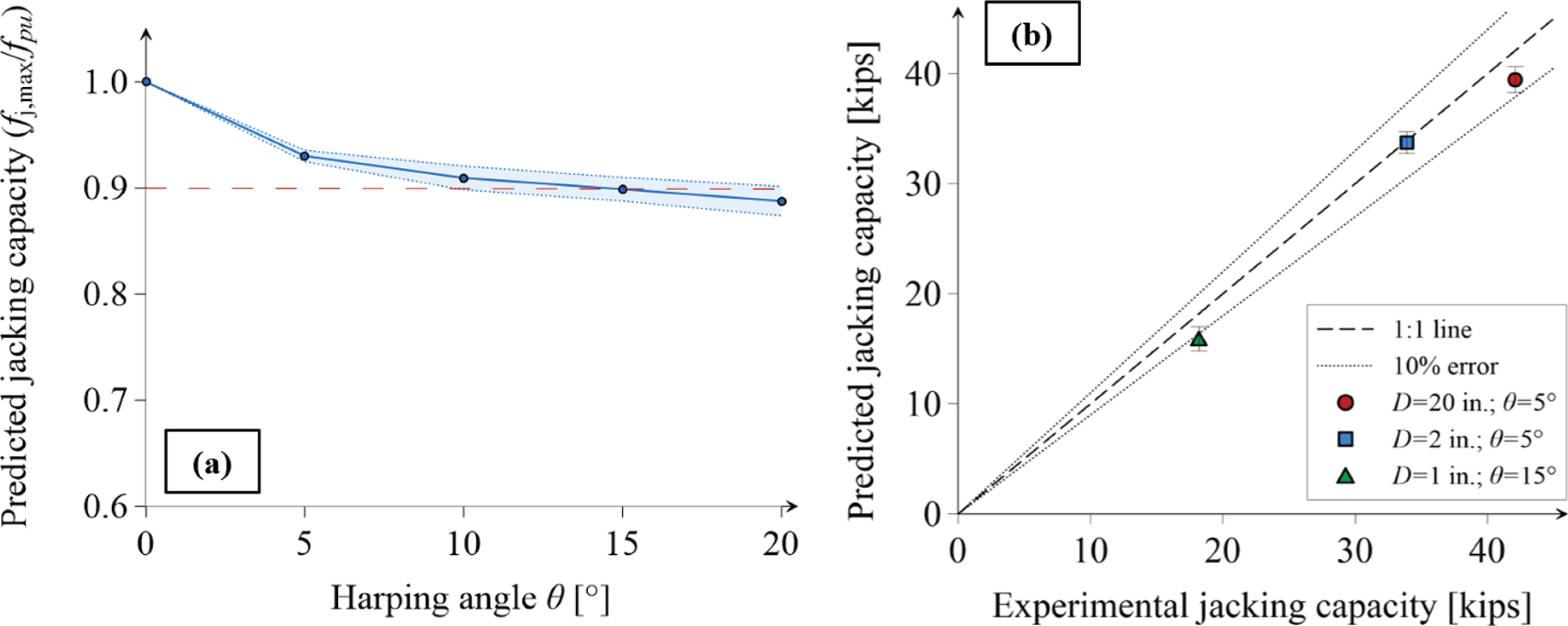
The results for the CS strand for different harping angles are presented in Figure 39a. It can be seen that up to a harping angle of 20°, the jacking capacity was reduced only by 10% to 12%. It coincides with the fact that harping CS strands is a common practice, and only a slight reduction of jacking capacity is expected. Note that according to ASTM A416, the minimum required ultimate strain (ε_pu) for CS is 0.035. However, laboratory test results indicate that the ultimate strain is usually higher than the minimum specified value. Using a higher ultimate strain based on test results would further increase the predicted jacking capacity; e.g., assuming ε_pu = 0.06, the predicted jacking capacity for a 20° harping angle is 93% of f_pu instead of 89%.

The FE model was further validated against the experimental data reported in Tahsiri and Belarbi (2022) for 0.6 in. CFRP seven-wire strand. Harping angles in the range of 5° to 15° and deviator diameters ranging from 1 in. to 20 in. were considered. The results of the breaking

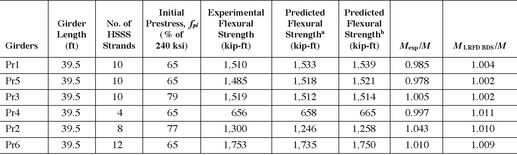
Note: For comparison purposes, the flexural strength was predicted using stress block factors α₁ and β₁ provided in LRFD BDS and stress block factors calculated using the general equations from Belarbi et al. (2019) (see Figure 38). The flexural strengths computed using both prediction methods show excellent agreement with test results and between the two methods as shown in Table 13.

a. Belarbi et al., 2019.

b. AASHTO, 2020 (LRFD BDS 9th).

Long Description.

The table summarizes flexural strength results for six girders, each 39.5 feet long. It includes the number of high-strength stainless steel strands, initial prestress as percent of 240 k s i, experimental flexural strength in kip-feet, and predicted strengths by Belarbi et al. 2019 and AASHTO Load and Resistance Factor Design 2020 methods. P r 1 with 10 strands at 65 percent prestress shows 1510 kip-feet experimental strength versus 1533 and 1539 predicted, yielding ratios of 0.985 and 1.004. P r 5 also with 10 strands shows 1485 kip-feet experimental, 1518 and 1521 predicted, with ratios of 0.978 and 1.002. P r 3 with 10 strands at 79 percent shows 1519 experimental, 1512 and 1514 predicted, with ratios of 1.005 and 1.002. P r 4 with 4 strands shows 656 experimental and nearly equal predicted values of 658 and 665, with ratios of 0.997 and 1.011. P r 2 with 8 strands at 77 percent prestress shows 1300 experimental, 1246 and 1258 predicted, giving the highest ratios of 1.043 and 1.010. P r 6 with 12 strands shows 1753 experimental, 1735 and 1750 predicted, with ratios of 1.010 and 1.009. The results confirm strong agreement between experimental and predicted strengths across all methods.

Long Description.

Two plots compare predicted and experimental jacking capacities of prestressing strands. Plot a on the left shows the predicted jacking capacity ratio on the vertical axis versus harping angle in degrees on the horizontal axis for carbon steel strands. The ratio decreases as the harping angle increases from 0 to 18 degrees, indicating reduced efficiency. A dashed line marks a baseline ratio of 0.9. Plot b on the right compares predicted versus experimental jacking capacities in kips for carbon fiber reinforced polymer strands. The diagonal solid line represents the 1 to 1 agreement line, while dashed lines indicate 10 percent error bounds. Data points include squares and triangles representing different strand diameters and angles. Most points fall within the error bounds, showing strong agreement between experimental and predicted capacities across the range of tested configurations.

load obtained in the experiments and predicted by the numerical model are shown in Figure 39b. A very good agreement between FE simulations and experimental data was achieved (less than 7% error). Therefore, it can be concluded that the created FE model sufficiently reflects the trend of jacking stress test results for harped strands with different deviator sizes and harping angles for both CS and CFRP strands.

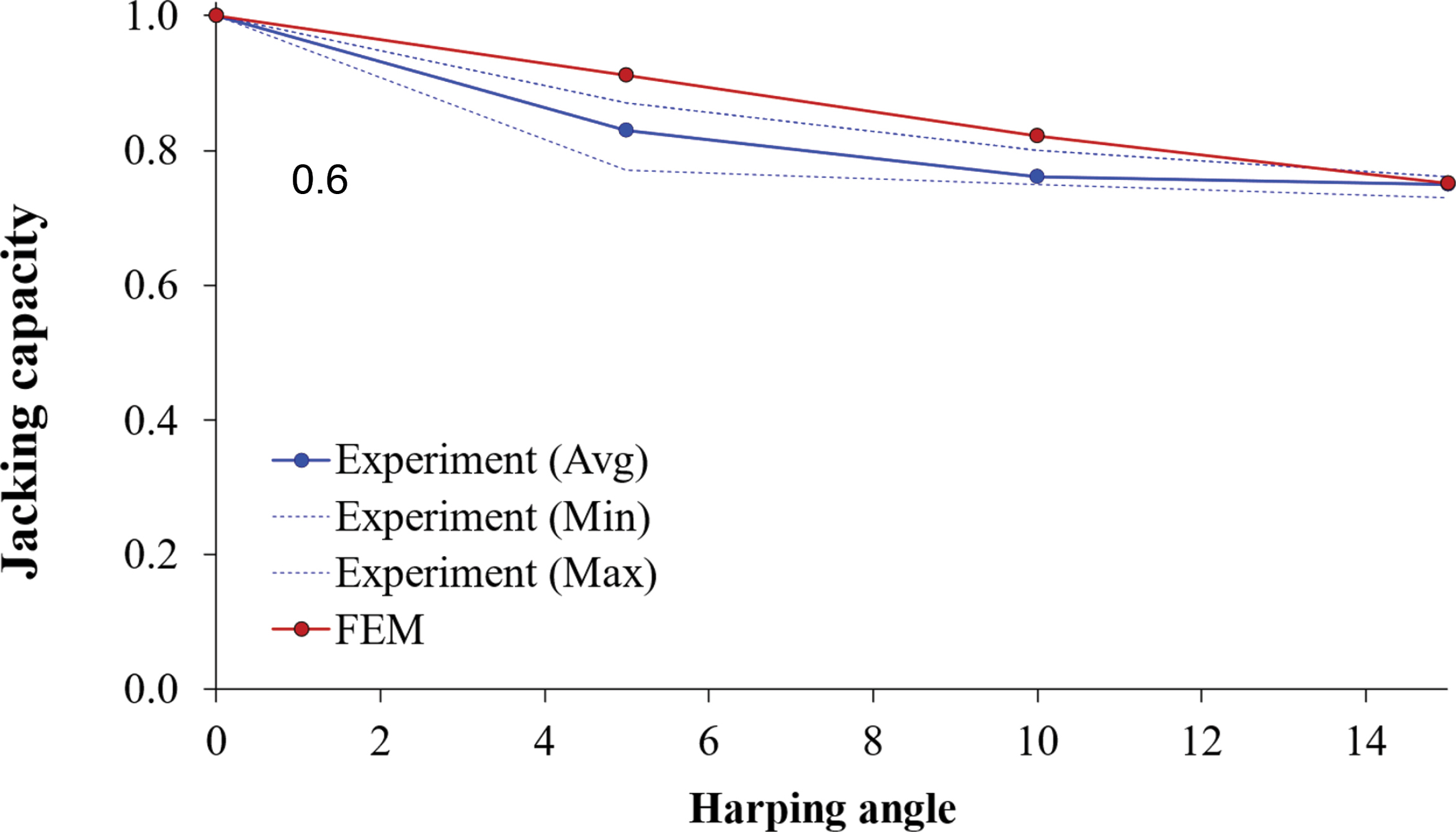
Finally, experimental results of the jacking capacity of SS strands are compared with FE model predictions as a function of harping angle in Figure 40. It can be seen that the updated constitutive model, including ductile damage of SS strands, drastically improved the match between experimental results and numerical predictions.

4.3 Transfer Length

In all simulations, the friction coefficient of 0.43 was utilized (the previously calibrated value for 0.6 in. CS strand). The friction coefficient, µ, for CS strands and concrete is usually assumed between 0.4 and 0.7 (0.4 is the most common value used). Prior to the experimental tests, comprehensive

Long Description.

The graph plots jacking capacity on the vertical axis from 0 to 1.0 and harping angle in degrees on the horizontal axis from 0 to 15. Four curves are shown: the experimental average, experimental minimum and maximum, and finite element method prediction. At 0 degrees, all curves begin near 1.0. As the harping angle increases, the jacking capacity decreases. At 5 degrees, the experimental average drops below 0.8, while the F E M prediction remains higher. At 15 degrees, all curves converge around 0.72. The graph shows a consistent trend of decreasing jacking capacity with increasing harping angle, with F E M results generally overestimating compared to experimental average but remaining within the experimental range.

FE analysis was performed using data from the literature to establish a friction coefficient of 0.43 for 0.60 in. CS strand (this value is close to the value commonly used in the literature).

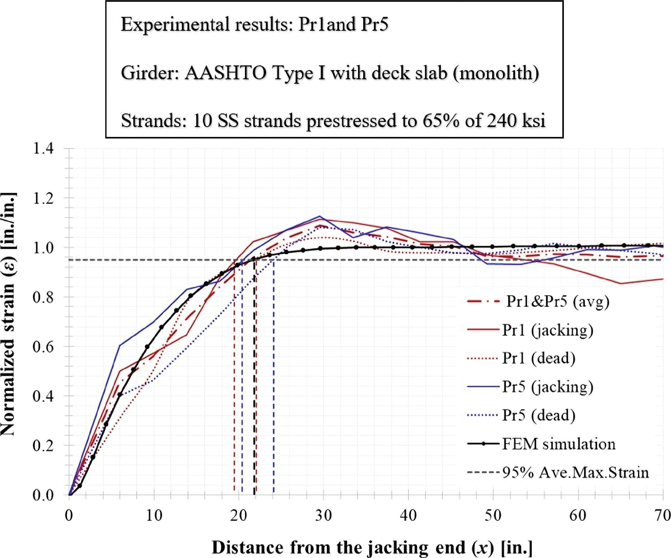
Preliminary calibration of the FE model for 0.62 in. diameter SS strands resulted in µ = 0.37 (Stefaniuk et al., 2025). Due to a lack of sufficient data in the literature for a friction coefficient for SS strands, additional validation was performed. Experimental data collected in this project were used for both SS and CS strands, which were found to have similar bond properties at 0.1 in. slippage according to ASTM A1081, as noted earlier in this report. These simulations focused on the large-scale girders that had been previously tested. The experimental results, specifically the normalized concrete strain along the beam (the strain data was normalized against the average maximum strain), were compared with the FE model for all the girders that measured strains along the girder to determine the transfer length. Strain data for Specimens Pr1 and Pr5 are presented in Figure 41 for both the jacking end and the dead end. More detailed results are provided in Appendix B.

It is important to note that in the FE model, no distinction was made between the jacking and dead ends; the variation in the figures is solely due to differences in experimental data. The plots in Figure 41 clearly illustrate that the FE model results closely match the experimental data.

The calibrated FE model showed excellent agreement with experimental data, accurately capturing the concrete strain profile near the girder ends and predicting transfer lengths with less than 10% error. This level of precision aligns with typical measurement uncertainty and repeatability, which is approximately 7% for identical girders.

4.4 Reliability Analysis

The purpose of the reliability calibration study was to ensure that the probability of failure, P_f, for beams designed using the proposed provisions is below the targeted acceptable risk levels as measured by the reliability index, β. Two reliability approaches, Monte Carlo simulations and the First Order Reliability Method (FORM), were used to assess the variability of the behavior of prestressed concrete elements with SS strands caused by known sources of uncertainty (namely, randomness inherent in material properties, M, and uncertainties attributed to fabrication tolerances, F) and, finally, the accuracy of the analysis model, P, and the applied loads. This study focused on the strength limit state.

Long Description.

The graph displays normalized strain on the vertical axis and distance from the jacking end in inches on the horizontal axis, ranging from 0 to 70 inches. The data corresponds to specimens P r 1 and P r 5, each with 10 stainless steel strands prestressed to 65 percent of 240 k s i in an AASHTO Type 1 girder with monolithic deck slab. Separate lines represent jacking and dead end measurements are included for both specimens. An average curve for P r 1 and P r 5 is also included. A horizontal dashed line marks the 95 percent average maximum strain. A simulation curve based on finite element modeling is also plotted. All curves show that normalized strain increases from zero at the jacking end and reaches peak values between 20 and 30 inches before gradually decreasing and stabilizing. Vertical dashed lines indicate approximate transfer lengths. The simulation result closely follows the experimental trends, validating the observed strain behavior along the beam.

The calibration conducted in this study was based on the theory of structural reliability and followed the same framework used in the calibration of AASHTOʼs LRFD Bridge Design Specifications as reported in NCHRP Report 368: Calibration of LRFD Bridge Design Code (Nowak, 1999, p. 37) and several other AASHTO documents (Moses, 2001; Kulicki et al., 2006; Mlynarski et al., 2011). This section summarizes the reliability study. For more details about the reliability study, the reader is referred to Appendix D.

4.4.1 Design Space

To perform the calibration of design factors, a design space consisting of 96 prestressed concrete bridges with SS strands was selected and designed following the fundamental concepts of equilibrium and strain compatibility. Because the dominant failure mode is controlled by strand rupture for beams prestressed with SS strands, the compression block parameters α₁ and β₁ corresponding to a maximum concrete strain, ε_cc, that is less than the ultimate concrete compressive strain, ε_cu, of 0.003 are used in the design. Three bridge attributes were considered in the design space: girder spacing, span length, and girder type. In determining the number of required strands, each case was designed for a midspan section to satisfy LRFD BDS provisions, namely Strength I, Service I, Service III, and minimum reinforcement requirements. Three groups of precast sections were included in the design space, namely AASHTO standard beam sections (e.g., Type II or BT-72), wide-flanged beam sections (e.g., FIB-45), and a group of special sections [NEXT, FSB, and AASHTO Box Beams (BB)].

An 8.0 in. thick reinforced concrete deck and a 1.0 in. haunch on top of the girderʼs top flange were assumed for all bridges, except for the AASHTO BB and FSB sections, where the deck thickness was taken as equal to 5.0 and 6.0 in., respectively, and four bridge cases with full-depth precast NEXT beams. The girders were designed to resist HL-93 loading and a future wearing surface load equal to 24 psf. Material properties considered in the study were an assumed concrete compressive strength of 8.5 ksi (6.8 ksi at transfer) for the precast beams and 4.0 ksi

for the deck concrete. Longer span cases (i.e., L = 140 ft and L = 170 ft) required higher concrete strengths and deck thicknesses. Grade 240 SS prestressing strands were used in the design of all girders in the design space. In total, 96 bridges were included in the design space.

4.4.2 Flexural Design and Analysis of Bridges in Design

4.4.2.1 Design

A spreadsheet was developed for the design of the bridges in the design space considering the aforementioned LRFD BDS limit states and minimum reinforcement requirements for a midspan section. The reader is referred to Appendix D for the details of the designed bridges including moment demands due to wearing surface (M_DW), components (M_DC), live load including dynamic allowance (M_LL+IM), and the main design details including the nominal moment of the designed beams (M_n); the initial prestressing force (P_pi); the eccentricity of the selected strand configuration at midspan (e_mid); and the curvature at failure of the design beams (κ). A ratio of the live load demand to the total demand for bridges in the design space covers a range from 0.29 to 0.62. This range plus the various design parameter ranges provide information about the reliability of the proposed design equations over a wide range of design scenarios that the proposed design requirements address.

4.4.2.2 Analysis

The flexural behavior of SS prestressed concrete elements was studied using a detailed fiber section model based on the well-established concepts of equilibrium and compatibility. The model thoroughly considers parameters affecting the behavior of prestressed concrete members including mechanical properties of available strands, prestress losses, stress level, and construction sequence. Three stages in the life of a prestressed concrete bridge girders are considered, namely (1) noncomposite girder only stage, (2) noncomposite beam after casting deck fresh concrete, and (3) composite beam after deck concrete sets. The model was used for generating the moment–curvature (i.e., M–κ) relations for all SS prestressed bridges in the design space. M–κ relations were generated using nominal material and fabrication parameters as well as randomly generated values. The former is for assessing behavior, while the latter is for establishing the statistical information used in the reliability study.

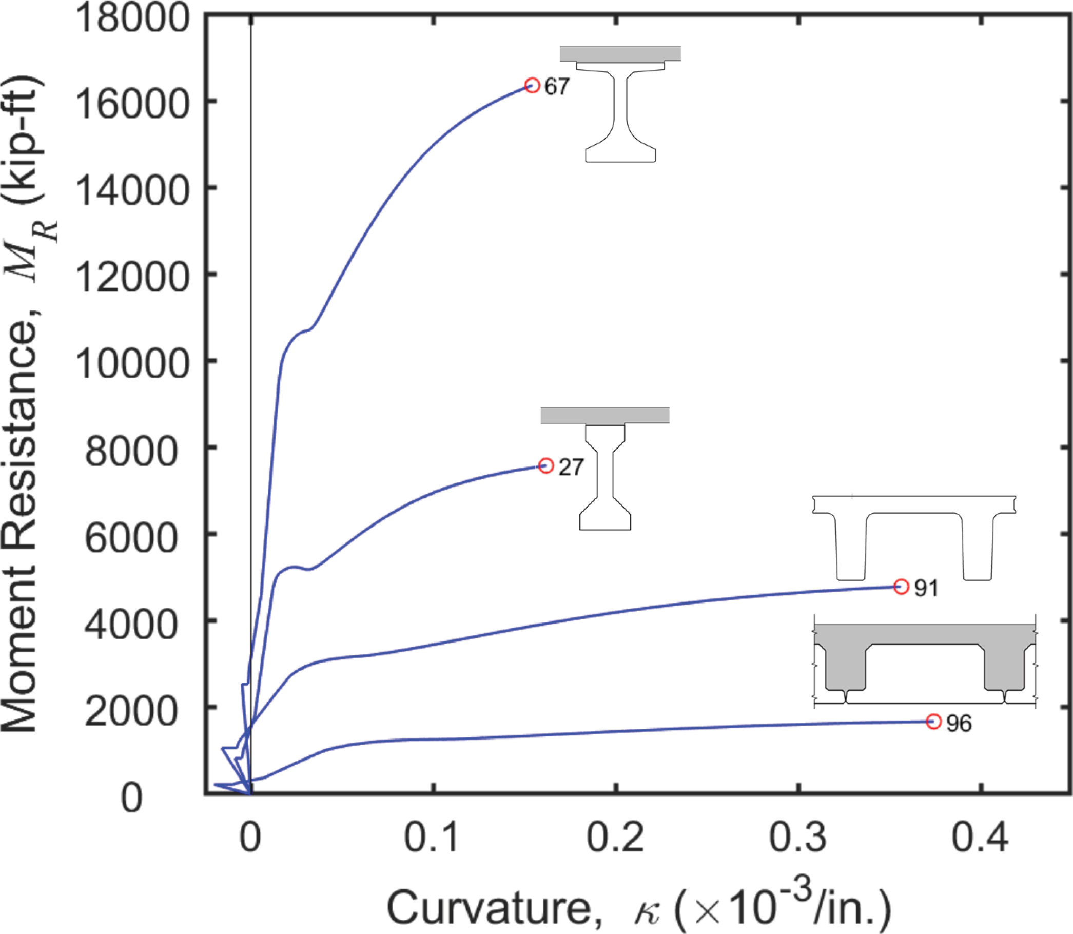
The M–κ relations for the nominal section properties were then used to study the load-deflection (i.e., P-∆) behavior of each beam considering the nonlinearities exhibited in the M–κ relations. The flexural rigidity, EI, was determined from the M–κ relations for each element in a beam stiffness model assuming simply supported bridge configurations. Figure 42 shows the M–κ relations for four sample bridges of different shapes from the design space. The number provided next to each M–κ relation is the case number. The reader is referred to Appendix D for more information about these cases.

4.4.3 Design Parameters

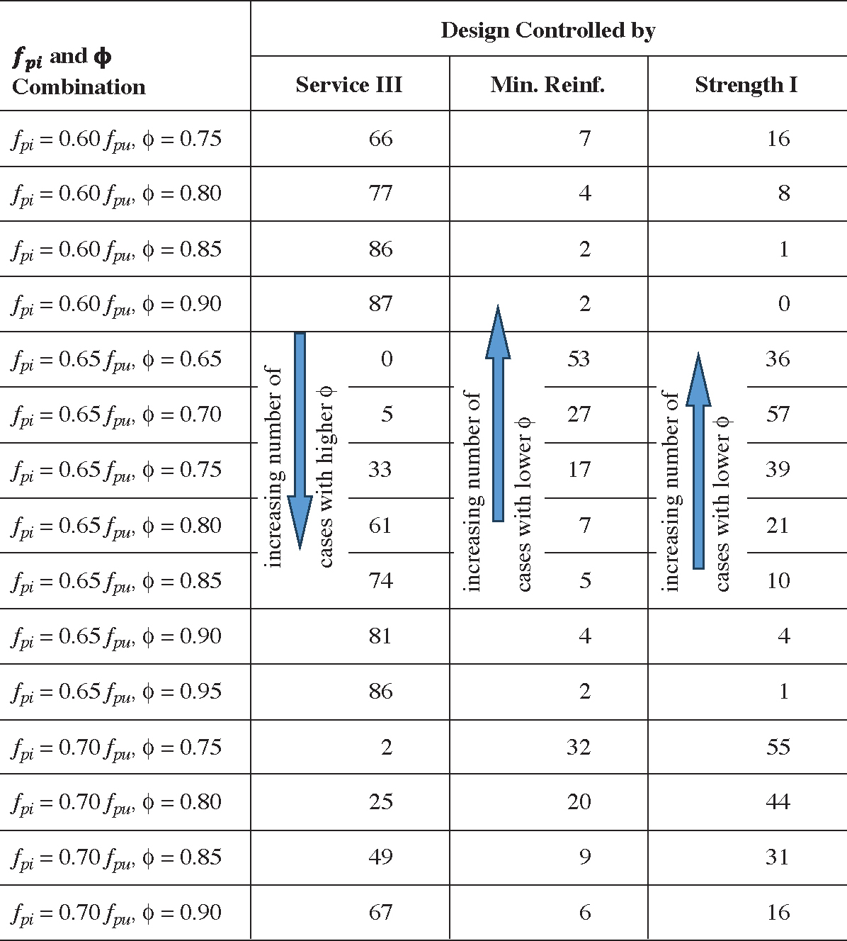
Bridges in the identified design space were used to investigate two design parameters, namely, initial prestress level, f_pi, and resistance factor, ϕ. All bridges were redesigned for ϕ = 0.65 to 0.95 in 0.05 increments for an initial prestress level, f_pi = 0.65f_pu, and ϕ = 0.75 to 0.90 for f_pi = 0.60f_pu and 0.70f_pu. This brings the total number of design combinations to 15.

The main conclusion from this investigation is that increasing the resistance factor, ϕ, causes more cases to become controlled by Service III limit state or minimum reinforcement requirements as a result of the smaller nominal resistance, M_n, is required to satisfy Strength I limit state. This trend is true for all f_pi values as can be seen in Table 14. These observations imply that

SS-prestressed beams, like CS-prestressed beams, will have reserve strength beyond the Strength I limit state requirements in many cases. Nevertheless, this reserve strength will not be taken into account in the reliability calibration as discussed later. The values used for ϕ and f_pi also have an impact on the deflection and the total strain energy at failure. For more details, the reader is referred to Appendix D.

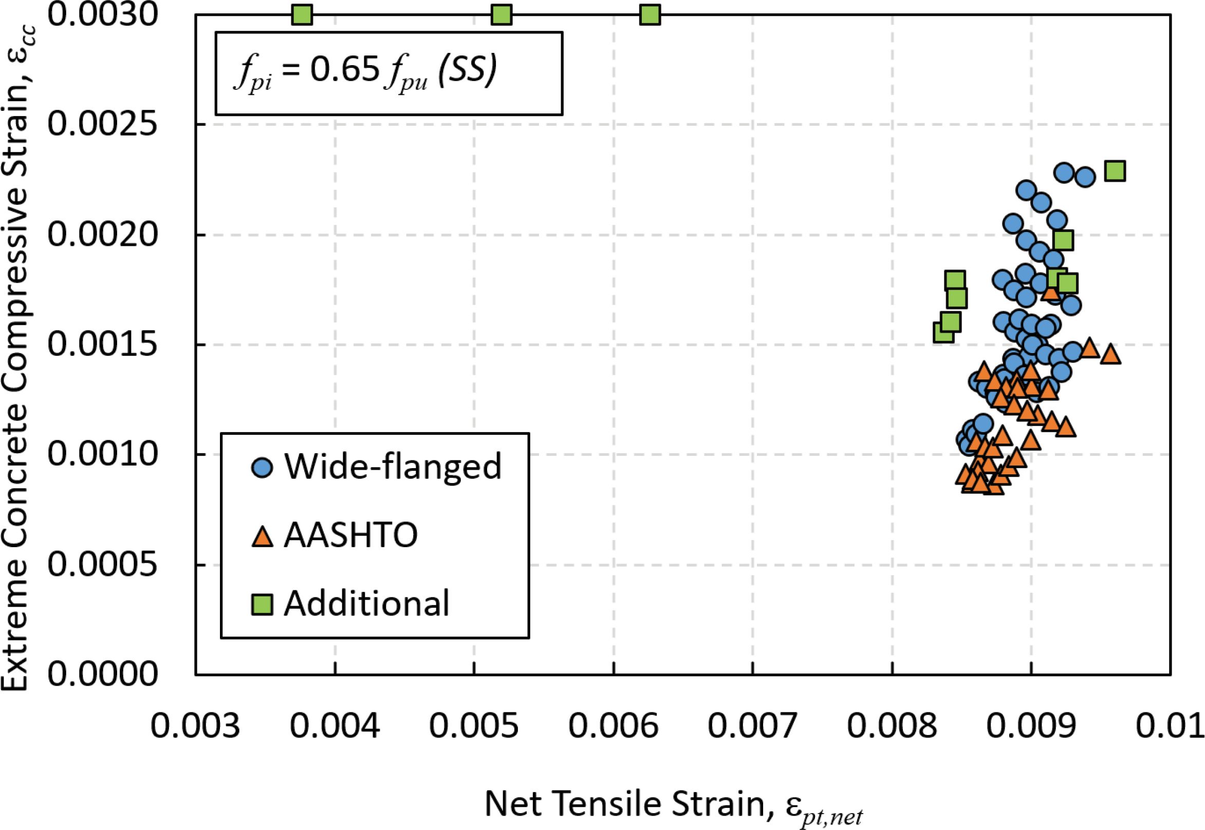
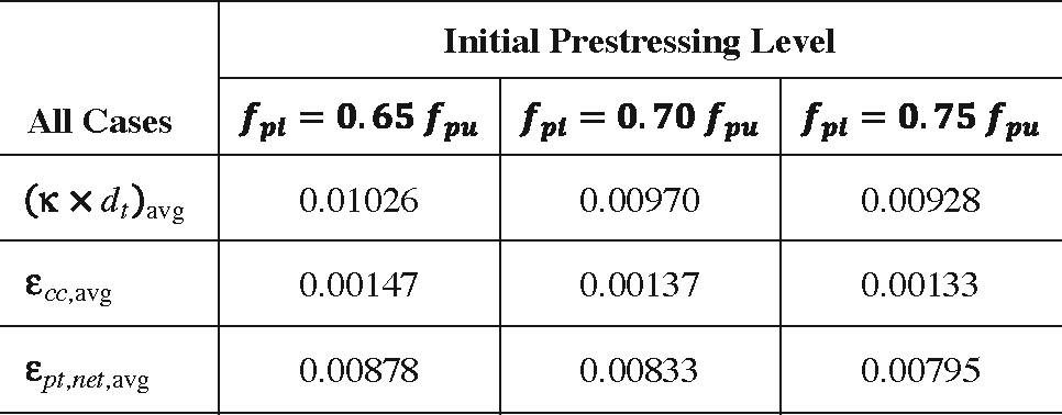
Figure 43 shows a plot of the extreme concrete compression strain, ε_cc, and net strand strain ε_pt,net at failure, which illustrates that the vast majority of bridges in the design space fail by strand rupture (all except for the three FSB cases) regardless of the controlling design provision. From these strains, the curvature, κ, can be calculated and normalized for the different depths by multiplying it by the effective depth of the strands (i.e., κ × d_t). Table 15 lists the average values of the normalized curvature, κ × d_t, extreme concrete compression strain, ε_cc, and net strand strain ε_pt,net at failure for the three groups of beam sections in the design space. The initial prestress level, f_pi, also affects the beamʼs curvature, κ, at failure. By normalizing the curvature for different beam depths, comparisons with the corresponding value for other strand alternatives can be made. For example, in AASHTOʼs LRFD Bridge Design Specifications, 9th ed. (AASHTO, 2020) (LRFD BDS 9th), CS strands are considered to provide a “desirable” design when the normalized curvature, κ × d_t, is equal to or greater than 0.008 (ε_cu + TCL = 0.003 + 0.005), where TCL is the tension-controlled strain limit (i.e., a tension-controlled failure). Tension-controlled carbon steel prestressed concrete flexural elements are designed with a resistance factor ϕ = 1.0. It can be seen from Table 15 that the normalized curvature, κ × d_t, would be classified as tension-controlled according to LRFD BDS, i.e., κ × d_t > 0.008 for all initial prestressing levels.

Long Description.

The graph plots extreme concrete compressive strain on the vertical axis from 0 to 0.0030 and net tensile strain on the horizontal axis from 0.003 to 0.01. Data points represent three categories: wide-flanged sections as circles, AASHTO girders as triangles, and additional cases as squares. All data points correspond to an initial prestress level of 0.65 times the ultimate strand stress. Wide-flanged and AASHTO data cluster between 0.008 and 0.009 net tensile strain and between 0.0010 and 0.0020 compressive strain. Additional cases show higher compressive strain, up to 0.0030, while spanning a wider range of tensile strain. The distribution highlights variations in failure behavior across different girder types and section configurations under the same prestress level.

Long Description.

The table shows average values of curvature times tensile depth, extreme compressive strain, and net tensile strain for all cases under three initial prestressing levels: f p i equals 0.65 f p u, f p i equals 0.70 f p u, and f p i equals 0.75 f p u. For f p i equals 0.65 f p u, the average curvature times depth is 0.01026, compressive strain is 0.00147, and net tensile strain is 0.00878. For f p i equals 0.70 f p u, the average values are 0.00970, 0.00137, and 0.00833, respectively. For f p i equals 0.75 f p u, the values are 0.00928, 0.00133, and 0.00795. As the prestressing level increases, all three metrics slightly decrease, indicating a trend of reduced strain and curvature at higher prestress levels.

It can be seen from Table 15 that the normalized curvature, κ × d_t, would be classified as tension-controlled according to LRFD BDS, i.e., κ × d_t > 0.008 for all initial prestressing levels.

4.4.4 Resistance Model

Three primary sources of uncertainty influence the variability of resistance models: material variability (M), fabrication tolerances (F), and analysis accuracy or professional factor (P). In this study, all three are modeled as random variables. The resulting resistance, represented as the random variable R, can be expressed as:

where R_n is the nominal resistance as obtained from the proposed design expression. The details of each one are described next.

4.4.4.1 Statistical Properties of Resistance Parameters

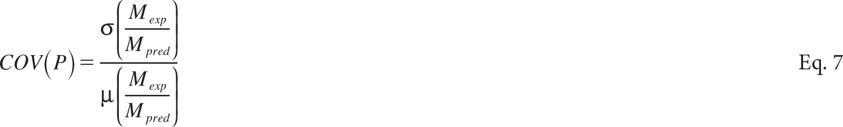
Twenty experimentally tested specimens were compiled in the database, 12 of which are specimens built with AASHTO Type I and Type II beams with composite decks and eight specimens with rectangular sections. The experimental database consisted of results from beams tested through research projects funded by GDOT (Paul et al., 2017), FDOT (Al-Kaimakchi and Rambo-Roddenberry, 2021), and specimens tested as part of this project. The main attributes of experimentally tested beams can be found in Appendix D. These specimens failed by strand rupture for all beam specimens (12) and by concrete crushing for the shallower specimens. The results from the analysis model for predicting the flexural capacity, M_pred, were compared with the experimental capacities, M_exp, reported by the respective researchers. The statistics of the M_pred/M_exp ratio were calculated to obtain the bias of the professional factor, λ_P, and its coefficient of variation, COV(P):

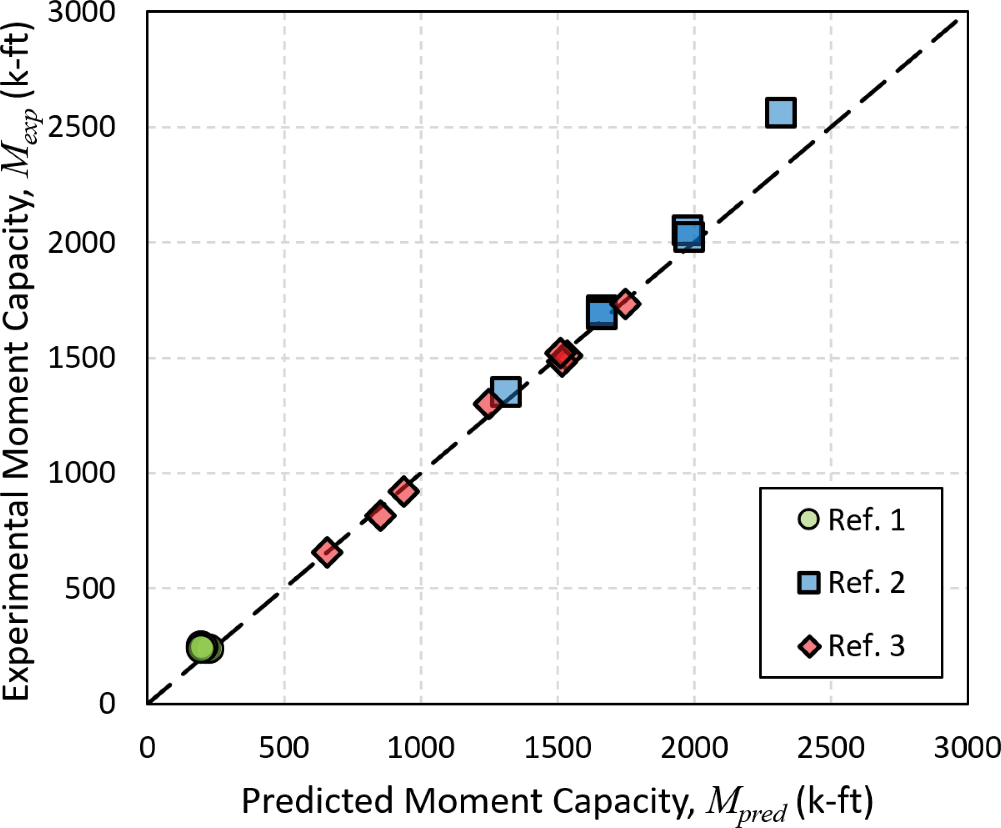
Figure 44 shows a comparison of experimental and predicted moment capacity for all 20 specimens. The results were separated based on the observed modes of failure (i.e., strand rupture and concrete crushing). The results show that the scatter for the strand rupture mode of failure [COV(P) = 3.38%] is less than the scatter for the concrete crushing mode of failure [COV(P) = 10.81%]. This is expected as concrete crushing is typically inherently more random than strand rupture, which is mechanistically easier to predict. This higher scatter for the concrete crushing mode of failure is offset by a higher bias, λ_P, of 1.125, that exceeds the bias for the strand rupture mode of failure, λ_P = 1.025. The corresponding bias, λ_P, and coefficient of variation, COV(P), for all cases are equal to 1.065 and 8.74%, respectively. A goodness-of-fit analysis was conducted to select the most suitable distribution type for the professional factor, P, which revealed that a lognormal distribution is a better fit for the results in the database.

Variabilities in material properties were also included in the reliability study. Uncertainties in concrete compressive strength, f′_c, was adopted from Nowak and Szerszen (2003) where the

Long Description.

The graph compares experimental moment capacity, labeled M sub experimental in kip-feet on the vertical axis from 0 to 3000, with predicted moment capacity, labeled M sub predicted in kip-feet on the horizontal axis from 0 to 3000. A dashed diagonal line represents a 1 to 1 correlation. Data points cluster near the line, representing close agreement between predicted and experimental values. Points are differentiated by source: Reference 1, Reference 2, and Reference 3. Reference 1 includes 1 point, Reference 2 includes 5 points mostly above 1500 kip-feet, and Reference 3 includes multiple points below 1500 kip-feet. All data are approximate.

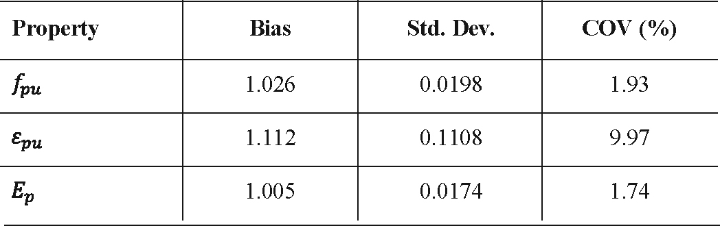
bias is a function of f′_c and the coefficient of variation is taken as equal to 10%. For SS prestressing strands, results from testing coupons from nine SS spools were analyzed statistically to estimate the variability inherent in their properties. The bias and coefficient of variation for the modulus of elasticity, E_p, rupture strain, ε_pu, and ultimate stress, f_pu were also assessed. Table 16 provides the bias, standard deviation, and the coefficient of variation for all three properties.

Fabrication tolerances were extracted from the literature for most design dimensions such as web width, b, and effective depth, d_p, and initial prestressing strain level, ε_pi. Other fabrication tolerances specific to SS strands were determined from the spools tested by Al-Kaimakchi and Rambo-Roddenberry (2021) and as part of this study. The nominal SS strand area, A_p, for 0.62 in. diameter strands was found to be almost consistent for all nine spools with little variability [i.e., bias, λ_Ap, equal to 1.022 and COV(A_p) equal to 2.05%]. These random variables were assumed to follow a normal distribution.

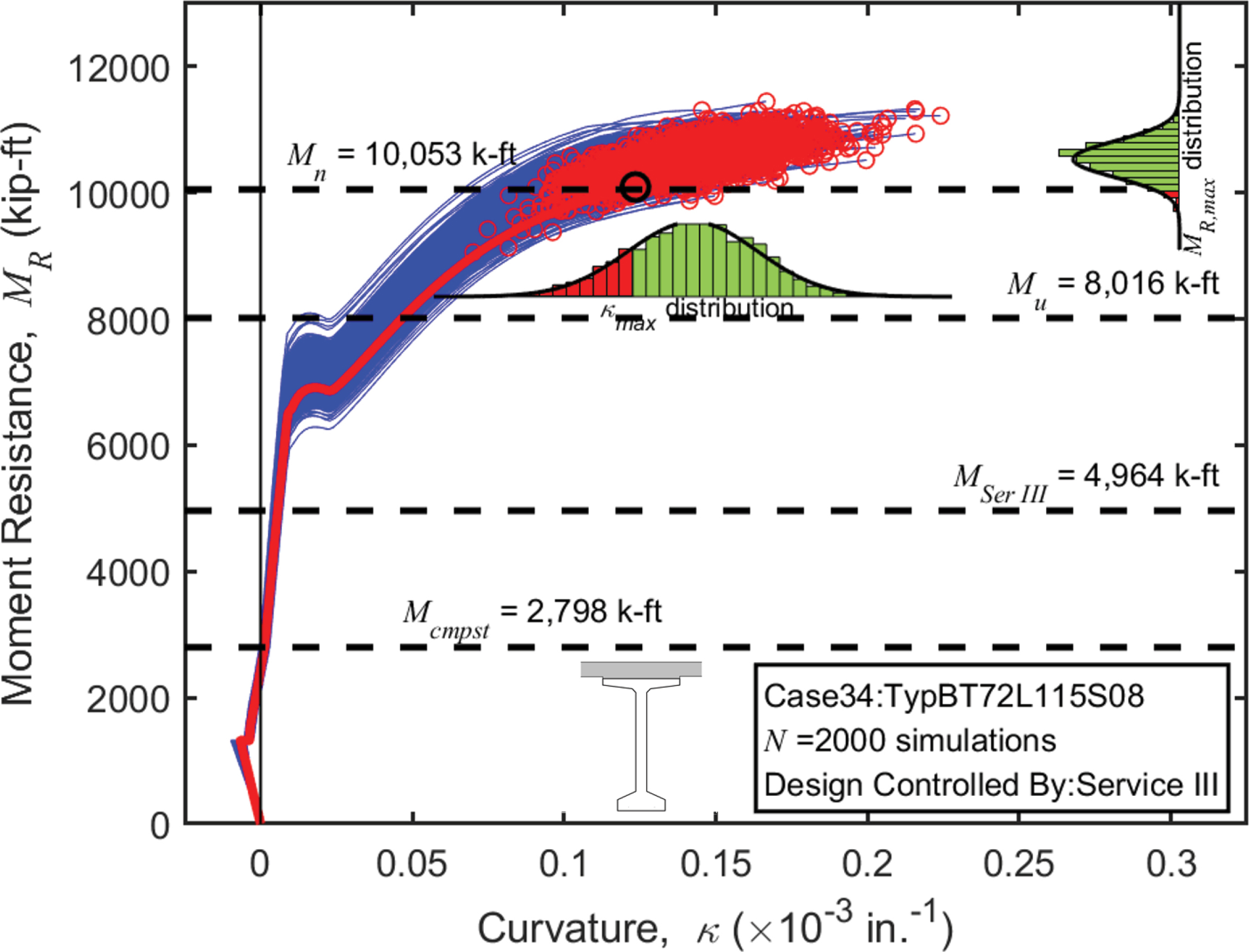
The uncertainty in the resistance model arising from material variability and fabrication tolerances was evaluated collectively through Monte Carlo simulations. The analysis involved generating random values for design equation parameters such as material properties, geometric dimensions, and initial prestress levels based on their defined statistical characteristics, discussed earlier. Figure 45 shows 2,000 variations of the moment–curvature relationships obtained

Long Description.

The table displays the statistical analysis results of mechanical properties for stainless steel prestressing strands. It includes three properties: ultimate tensile strength denoted as f sub p u, ultimate strain denoted as epsilon sub p u, and modulus of elasticity denoted as capital E sub p. For each property, the table lists its bias, standard deviation, and coefficient of variation. The bias values are 1.026 for f sub p u, 1.112 for epsilon sub p u, and 1.005 for capital E sub p. The corresponding standard deviations are 0.0198, 0.1108, and 0.0174, respectively. The coefficient of variation values are 1.93 percent, 9.97 percent, and 1.74 percent, respectively.

Long Description.

The graph depicts moment resistance versus curvature for Case 34, identified as Typ B T 72 L 115 S 0 8, based on 2000 simulations. The horizontal axis is labeled as curvature, kappa, in units of 10 to the power of negative 3 inches to the power of negative 1, ranging from 0 to 0.3. The vertical axis is labeled as moment resistance, M sub R, in kip-feet, ranging from 0 to 12,000. Multiple simulation curves are shown along with a distribution of R sub n, max, and kappa max. Several horizontal dashed lines mark key moments: M sub n equals 10,053 kip-feet, M sub u equals 8,016 kip-feet, M sub Ser 3 equals 4,964 kip-feet, and M sub cmpst equals 2,798 kip-feet. The design is noted to be controlled by Service 3. A bridge section shape is shown near the bottom of the graph.

for one of the bridge cases in the design space (Case 34 – TypBT72L115S08) given M and F uncertainties. Also shown in the figure is the M–κ relation obtained using the nominal beam property. The ultimate moment from each simulated moment–curvature is identified with a circle marker on the plots. Cumulatively, these points represent the randomness of the flexural capacity and associated curvatures due to material and fabrication tolerances. Also, in the figure, histograms of the failure point attributes (M_R,max and κ_max) are plotted. Of interest in this study is the histogram of M_R,max, which represents the randomness of the flexural capacity due to material and fabrication tolerances. From these Monte Carlo simulations, the bias, λ_MF, and coefficient of variation, COV(MF), due to material and fabrication tolerances were calculated for all cases in the design space. The mean, µ, and standard deviation, σ, and the associated bias, λ, and coefficient of variation, COV, at failure for both the flexural capacity, M_R,max, and for the curvature at failure, κ_max, for each of the analyzed cases can be found in Appendix D. From these results, it was concluded that the overall bias, λ_MF, is equal to 1.04 and the overall coefficient of variation, COV(MF), is equal to 2.7%.

4.4.5 Load Model

This study used published and well-established statistical characteristics for highway loads that were used in the calibration of the LRFD BDS. The bias and coefficient of variation for load effects used in the study were taken from Nowak (1999, p. 37).

The accuracy of the girder distribution factor typically used in the design of bridges was accounted for using a random variable, ξ_GDF. The bias, λ_ξGDF, and coefficient of variation, COV(ξ_GDF), taken from NCHRP Report 592 (BridgeTech Inc. et al., 2007), are equal to 1.109 and 10.4%, respectively, for interior girders.

4.4.6 Calibration of Resistance Factor, ϕ

4.4.6.1 Strength Limit State Function

The limit state function for the Strength I limit state, g_Str.I, is given in Eq. 8. It represents the difference between the resistance and the load demands in a design equation for a certain structural element considering the uncertainties on both the demand and resistance side. This

includes the statistical characteristics for the sources of uncertainties (professional factor, P; material variabilities, M; fabrication tolerances, F) on the resistance side, and the uncertainties associated with dead and live loads published in the literature.

where M_R is the random variable representing the flexural resistance and M_DC, M_DW, and M_LL+IM are the random variables representing the load demands due to component dead loads, wearing surface dead loads, and live load plus impact, respectively. The random variable ξ_GDF was also included to account for the uncertainties introduced by the AASHTO girder distribution factor formulas that were introduced earlier.

4.4.6.2 Reliability Analysis Results

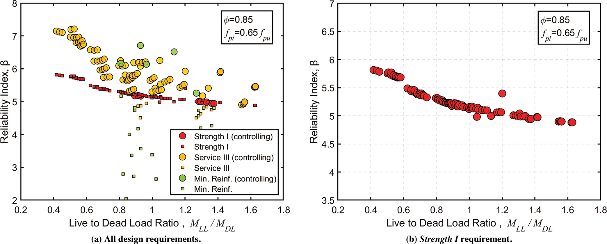
The β values determined using FORM are plotted in Figure 46a for the recommended resistance factor, ϕ. Three sets of β values are plotted corresponding to the Strength I and Service III limit states and minimum reinforcement requirements. As can be seen in Figure 46a, Strength I limit state controls the design for only a small number of bridges in the design space. Increasing ϕ reduces the number of cases controlled by Strength I limit state as Service III becomes the controlling limit state.

While the reserve strength resulting from Service III and minimum reinforcement requirements beyond Strength I requirements are generally welcome, the calibration of the resistance factor, ϕ, was conducted for the Strength I limit state regardless of these additional capacities. Figure 46b shows a plot of the β values specifically obtained from Strength I limit state designs for ϕ = 0.85 and f_pi = 0.65f_pu. It can be seen that all β values exceed the AASHTO-LRFD target reliability index, β_target, of 3.5. Since SS is a new construction material, it is prudent to consider a higher target reliability index. Furthermore, the limited rupture strain for SS strands (~1.4%) is far less than the strain at failure for CS strands (~4%). The structural engineering community agrees that different provisions and failure modes should be assigned different risks of failure. Allen (1992) suggested that β_target should reflect element behavior, system behavior, inspection level, and even traffic category. Therefore, it is recommended that a ϕ value of 0.85 is the appropriate choice for Strength I design of tension-controlled structural elements.

Long Description.

Two plots display the relationship between the reliability index, beta, and the live-to-dead load ratio, M sub LL over M sub DL, for bridge cases in the design space. The left plot includes all design requirements with separate marker styles indicating which requirement controls each case: Strength 1, Service 3, or minimum reinforcement. Marker shapes distinguish controlling from non-controlling cases. A decreasing trend in beta with increasing M sub LL over M sub DL is visible. The right plot focuses only on cases controlled by the Strength 1 requirement, showing a consistent decline in beta as M sub LL over M sub DL increases. Both plots use phi equal to 0.85 and initial prestress f sub pi equal to 0.65 times f sub pu.

4.4.6.3 Defining Tension- and Compression-Controlled Strain Limits

The recommended ϕ value of 0.85 is appropriate for the bridges in the design space whose failure mode was dominated by strand rupture that would be classified as tension-controlled in LRFD BDS, as discussed earlier (see Figure 43). Since the LRFD BDS specifies a ϕ value of 0.75 for compression-controlled designs, the transition zone must be defined between the recommended ϕ value of 0.85 for tension-controlled designs to the current value of 0.75 for compression-controlled designs. Defining this transition zone requires two strain limits: the compression-controlled strain limit (CCL) and the tension-controlled strain limit (TCL).

In the LRFD BDS, the CCL and TCL are given in terms of the net tensile strain, with values of ε_pt,net = 0.002 and 0.005, respectively. Historically, the CCL was set to 0.002, which is almost equal to the yield strain for Grade 60 steel reinforcement. The ACIʼs 2025 Building Code for Structural Concrete, ACI 318-25 (ACI Committee 318, 2025), changed the CCL to equal the yield strain, ε_ty, of whatever steel grade is used, and the TCL was taken as equal to CCL plus an additional strain of 0.003 such that cracking and deformations would provide ample warning prior to failure.

For CS strands, all flexural designs would have an ε_pt,net several times larger than the TCL = 0.005 in the current LRFD BDS. For SS strands, ε_pt,net at failure is in the range of 0.008 (see Figure 43), which is lower than the corresponding values for CS strands. To differentiate between the two modes of failure and to define an appropriate transition zone, it is recommended that the CCL be equal to ε_pt,net corresponding to a total strand strain equal to the yield strain for the SS strands. Therefore, the total strand strain, which is equal to the summation of the effective strain, ε_pe, and the net tensile strain, ε_pt,net, is set equal to the yield strain, or:

For f_pi = 0.65 f_pu, the average effective strain, ε_pe, for bridges in the design space ranged between 0.0052 and 0.0059 is with an average of 0.0056. For a SS strand yield strain, ε_py, equal to 1.0%, the ε_pt,net is roughly equal to 0.0045. Thus, a value of 0.0040 for the CCL, which leads to an earlier transition to a compression-controlled ϕ value of 0.75 than is currently in LRFD BDS. The TCL was determined in a manner similar to the one adopted by LRFD BDS and ACIʼs 2019 Building Code Requirements for Structural Concrete (ACI Committee 318, 2019) (ACI 318-19), where TCL is taken as CCL plus a strain of 0.003.

This would result in a TCL of 0.007. A limit of 0.0075 for TCL was selected in light of the fact that test results for several shallow beams in the literature that failed by concrete crushing would be in the transition zone and not in the tension-controlled region. See Figure 43 where three test results from the literature had concrete crushing failures at net strains between 0.0038 and 0.0063 with an average of about 0.0051.