Designing for Target Speed, Volume 1: Operating Speed and Road Elements (2026)
Chapter: Appendix D: Development of Analytical Approach
APPENDIX D. DEVELOPMENT OF ANALYTICAL APPROACH
As the information in the literature review indicates, there is a wide variety of factors that potentially influence operating speed, and subsequently target speed, that could be included in a thorough analysis, and those factors have different methods available to model them and investigate their relationships to speed. To investigate the effects of those various factors on operating speeds and to explore potential analyses approaches, the research team considered multiple modeling and analysis strategies to identify the most appropriate modeling approach as well as the variables most suitable for investigation.
DEVELOPING PRELIMINARY MODELS FOR OPERATING SPEED ANALYSIS
The main objective of this effort was to develop models for connecting operating speeds with road factors to understand and form relationships between operating speeds and those potential predictors for target speed selection.
The research team employed ANCOVA models that include both categorical/discrete factors and continuous covariates as predictors to explore the relationships among variables based on the dataset consisting of speed variables and many (40+) candidate predictor variables obtained from 636 sites located in Austin and San Antonio, Texas, as part of previous projects that collected datasets similar to those desired for NCHRP 15-76. The ANCOVA models can be viewed as normal linear regression models. Under the ANCOVA model, the interpretation of coefficients are straightforward and intuitive and the estimated regression coefficients represent the effect sizes of predictors. The ANCOVA models have been extensively used to assess the effects of various factors or covariates on the response variable when the relationship between the predictors and the response variable is deemed to be linear (as is or after applying appropriate transformations).
PHASE I EVALUATION OF PRELIMINARY MODELS AND DATA FOR SPEED ANALYSIS
The team supplemented available datasets with additional data such as census data to explore the feasibility of the methodology along with identifying whether some of the factors could be eliminated or should be emphasized during site selection.
Among several site-level operating speed measures (e.g., average speeds, 85th percentile speeds, standard deviation of speeds, etc.), the team used average speeds (denoted by SpdAve) as a response variable to explore the relationship among operating speeds and various roadway, roadside, and non-roadway factors. Table D-1 shows the list of variables selected for use in the analysis, including the roadway characteristics, the traffic characteristics, traffic control devices present, operating speed, roadside characteristics, and relevant non-roadway features. Table D-2 shows the summary statistics of those variables. Note that not all potential predictors in Table D-2 may have a significant relationship with SpdAve. Also, some predictors may be highly correlated, which leads to the collinearity problem in parameter estimation if included simultaneously (Spiegelman et al. 2010).
To develop appropriate parsimonious models (having important predictors), the team performed variable selection on potential predictors in Table D-2. The stepwise (forward, backward, or mixed) model selection procedure available in the statistical package JMP was utilized to perform variable selection with different selection criteria such as Bayesian Information Criterion (BIC), Akaike’s Information Criterion (AIC), corrected Akaike’s Information Criterion (AICc), p-value threshold, adjusted R2, or Cp, consistent with the method described by Spiegelman et al. (Spiegelman et al. 2010). The team used one of the following three stopping rules in implementing a stepwise model selection procedure in JMP: (a) p-value threshold, (b) minimum AICc, and (c) minimum BIC. Both AICc and BIC are penalized-likelihood criteria for model selection that balance the choice of model by adding a penalty for the number of predictors used to the residual sum of squares. Although a lower AICc or BIC means a better model, a simpler model can be selected by the principle of parsimony whenever there is not much difference in AICc (or BIC) values among competing models. Note that the best choice of a model may also depend on how useful the model is in the given context, not just on statistical model selection criteria.
Seven models for SpdAve, developed by Stepwise Fit in JMP with different stopping rules in combination with forward, backward, or mixed direction, are presented following Table D-2. The following sections present the results for each of the seven models, which are then followed by a summary of the findings.
Table D-1. Description of variables used in the preliminary analysis.
| Variable | Description |
|---|---|
| SpdAve | Average speed (mph) |
| Bike_1yes | Bicycle lane present: 1=yes, 0=no |
| BldHt1to4 | Typical height of adjacent buildings (number of stories), on a 1-4 scale (1=no buildings, 2=1 story, 3=2 or 3 stories, 4=more than 3 stories) |
| BldSet1to4 | Building setback (ft), on a 1-4 scale (1=no buildings within 100 ft, 2=buildings within 50-100 ft, 3=buildings within 20-50 ft, 4=buildings less than 20 ft) |
| CLmark | Center line marking presence: 1=yes, 0=no, 2=median |
| Curb_1yes | Curb and gutter present on segment: 1=yes, 0=no |
| Develop | Adjacent land development: Com/Ret/Ind, Residential, Rural/Parks |
| DrvUsigPerMileBoth | Driveways/unsignalized intersections per mile in both directions |
| ELmark | Edge line marking presence: 0, 1, or 2 sides of the street (use 1 for only side of street with direction of speed data, use 1.5 for only opposite side |
| Fence1to3 | Fence characteristics, based on a 1-3 scale (1=no fence or minimal fencing, 2=Solid/privacy fence (e.g., wood, stone, brick) 10-20 ft from road, 3 = Fence within 10 ft of road) |
| Horz_1tan | Horizontal alignment: 1=straight(tangent), 0=some horizontal curvature (HC) |
| LaneWidth | Typical or average lane width for the segment (ft) |
| Median | Type of median: none, TWLTL, raised |
| MedWidth | Typical or average median width for the segment (ft) |
| NumLanes | Number of lanes |
| Park_1yes | On-street parking (either marked or unmarked): 1=yes or 0=no |
| PedAuto | Typical / average distance between the sidewalk and the automobile lane for the segment (ft) |
| PSL | Posted speed limit (mph) |
| Variable | Description |
|---|---|
| RoadSurf | Distance between the driving surface edges, calculated as ThrLaneDir*2*LaneWidth+MedWidth+2*ParkWidth+2*BikeWidth |
| RoadType | Cross-section: 2D, 2U, 3T, 4U, 4D, 5T, 6D |
| School0.5 | Is a school located within 0.5 mi of the site: 1=yes or 0=no |
| SchZone_1yes | School Zone presence: 1=yes, 0=no |
| Sidewalk_1yes | Sidewalk presence: 1=yes or 0=no |
| SidewalkSep_1yes | Is the sidewalk separated from the curb: 1=yes or 0=no |
| SignalPerMile | Number of signalized intersections along segment, including any signals at the begin or end of the segment, divided by the length of segment in miles |
| StFurn1to4 | Street Furniture characteristics, based on a 1-4 scale (1=no street furniture, 2=Isolated street furniture greater than 20 ft from road, 3=Isolated street furniture within 20 ft, 4=Outside dining (tables and chairs), benches, and/or many objects next to edge of street) |
| StTree1to3 | Street Trees characteristics, based on a 1-3 scale (1=no trees within 30 ft or isolated/small tree, 2=A few trees but generally spaced about 30 ft apart and 20 ft from street edge, 3=Large tree and/or multiple trees within 10 ft of street) |
| Vol_Day | Volume per day, both directions |
| CBSA_POP | Total population in core-based statistical area (CBSA) for the relevant census block group (CBG) |
| CBSA_WRK | Total number of workers that live in CBSA |
| COUNTHU10 | Housing units, 2010 |
| D1a | Gross residential density (HU/acre) on unprotected land |
| D1b | Gross population density (people/acre) on unprotected land |
| D3a | Total road network density |
| E_PCTLOWWA | % LowWageWk of total #workers in a CBG (work location), 2010 |
| HH | Households (occupied housing units), 2010 |
| P_WRKAGE | Percent of population that is working aged, 2010 |
| PCT_AO0 | Percent of zero-car households in CBG |
| PCT_AO1 | Percent of one-car households in CBG |
| PCT_AO2P | Percent of two-plus-car households in CBG |
| R_HIWAGEWK | # of workers earning $3333/month or more (home location), 2010 |
| R_LOWWAGEW | # of workers earning $1250/month or less (home location), 2010 |
| R_MEDWAGEW | # of workers earning > $1250/month but < $3333/month (home location), 2010 |
| R_PCTLOWWA | % LowWageWk of total #workers in a CBG (home location), 2010 |
| WORKERS | # of workers in CBG (home location), 2010 |
| NatWalkInd | National Walkability Index score for CBG. |
Table D-2. Summary statistics for variables used in the Phase I analysis.
| Variable | Variable Type | Minimum | Maximum | Mean | Std. Deviation |
|---|---|---|---|---|---|
| SpdAve | Numerical | 10.92 | 47.28 | 27.99 | 6.86 |
| Bike_1yes | Dichotomous | 0 | 1 | 0.20 | 0.40 |
| BldHt1to4 | Numerical | 1 | 4 | 2.05 | 0.69 |
| BldSet1to4 | Numerical | 1 | 4 | 2.09 | 0.71 |
| CLmark | Numerical | 0 | 2 | 0.60 | 0.64 |
| Curb_1yes | Dichotomous | 0 | 1 | 0.95 | 0.21 |
| Develop | Categorical | ComRetlnd (89), Residential (513), Rural/Parks (4) | |||
| DrvUsigPerMileBoth | Numerical | 0 | 174.4 | 47.51 | 42.51 |
| ELmark | Numerical | 0 | 2 | 0.15 | 0.50 |
| Fence1to3 | Numerical | 0 | 3 | 1.30 | 0.63 |
| Horz_1tan | Dichotomous | 0 | 1 | 0.33 | 0.47 |
| LaneWidth | Numerical | 7 | 25 | 13.37 | 4.01 |
| Median | Categorical | Left-turn lane (6), None (537), Raised (43), TWLTL (50) | |||
| MedWidth | Numerical | 0 | 50 | 2.06 | 5.79 |
| NumLanes | Numerical | 2 | 6 | 2.25 | 0.69 |
| Park_1yes | Dichotomous | 0 | 1 | 0.31 | 0.46 |
| PedAuto | Numerical | 0 | 37 | 5.58 | 5.29 |
| PSL | Numerical | 25 | 40 | 30.33 | 4.44 |
| RoadSurf | Numerical | 18 | 100 | 38.94 | 12.51 |
| RoadType | Categorical | 2D (17), 2U (515), 3T (25), 4D (24), 4U (22), 5T (31), 6D (2) | |||
| School0.5 | Numerical | 0 | 1 | 0.79 | 0.41 |
| SchZone_1yes | Dichotomous | 0 | 1 | 0.09 | 0.29 |
| Sidewalk_1yes | Dichotomous | 0 | 1 | 0.63 | 0.48 |
| SidewalkSep_1yes | Dichotomous | 0 | 1 | 0.37 | 0.48 |
| SignalPerMile | Numerical | 0 | 13.7 | 1.50 | 2.45 |
| StFurn1to4 | Numerical | 1 | 4 | 1.33 | 0.73 |
| StTree1to3 | Numerical | 1 | 3 | 2.10 | 0.73 |
| Vol_Day | Numerical | 92 | 42695 | 5141.47 | 6790.58 |
| CBSA_POP | Numerical | 1716289 | 2142508 | 1736393.67 | 90430.37 |
| CBSA_WRK | Numerical | 753790 | 835629 | 757650.33 | 17363.68 |
| COUNTHU10 | Numerical | 242 | 4023 | 798.84 | 524.70 |
| D1a | Numerical | 0.11 | 16.66 | 3.22 | 2.31 |
| D1b | Numerical | 0.29 | 35.58 | 6.91 | 4.83 |
| D3a | Numerical | 1.75 | 39.89 | 16.96 | 7.26 |
| E_PCTLOWWA | Numerical | 0 | 0.85 | 0.27 | 0.13 |
| HH | Numerical | 229 | 3778 | 733.97 | 488.07 |
| P_WRKAGE | Numerical | 0.54 | 1.00 | 0.78 | 0.08 |
| PCT_AO0 | Numerical | 0 | 0.49 | 0.07 | 0.08 |
| PCT_AO1 | Numerical | 0.02 | 0.75 | 0.39 | 0.13 |
| PCT_AO2P | Numerical | 0.08 | 0.98 | 0.54 | 0.17 |
| R_HIWAGEWK | Numerical | 8 | 1290 | 334.99 | 214.43 |
| R_LOWWAGEW | Numerical | 16 | 442 | 170.96 | 72.41 |
| R_MEDWAGEW | Numerical | 10 | 713 | 276.54 | 129.81 |
| R_PCTLOWWA | Numerical | 0.14 | 0.5 | 0.22 | 0.05 |
| WORKERS | Numerical | 34 | 2257 | 782.48 | 352.57 |
| NatWalkInd | Numerical | 4.17 | 19.33 | 12.42 | 3.80 |
| Note: For dichotomous variables, ‘1’ indicates the presence of the feature and ‘0’ indicates its absence. | |||||
Model 1
Model 1 was obtained by forward direction with p-value stopping rule (Prob to Enter=0.25, Prob to Leave=0.1). The response variable is SpdAve. The following tables provide the results:
- Table D-3. Model 1 summary of fit.
- Table D-4. Model 1 analysis of variance.
- Table D-5. Model 1 parameter estimates.
- Table D-6. Model 1 effect tests.
Table D-3. Model 1 summary of fit.
| RSquare | 0.711036 |
| RSquare Adj | 0.694365 |
| Root Mean Square Error | 3.652032 |
| Mean of Response | 27.49714 |
| Observations (or Sum Wgts) | 606 |
| AIC and BIC | |
| AICc | BIC |
| 3329.067 | 3478.887 |
Table D-4. Model 1 analysis of variance.
| Source | DF | Sum of Squares | Mean Square | F Ratio |
|---|---|---|---|---|
| Model | 33 | 18772.097 | 568.851 | 42.6511 |
| Error | 572 | 7628.956 | 13.337 | Prob > F |
| C. Total | 605 | 26401.053 | <.0001* |
Table D-5. Model 1 parameter estimates.
| Term | Estimate | Std Error | t Ratio | Prob>|t| |
|---|---|---|---|---|
| Intercept | 20.856769 | 3.420987 | 6.10 | <.0001* |
| Bike_1yes | 1.6588535 | 0.468728 | 3.54 | 0.0004* |
| Horz_1tan | -1.24053 | 0.359155 | -3.45 | 0.0006* |
| LaneWidth | 0.1212042 | 0.048853 | 2.48 | 0.0134* |
| MedWidth | -0.150779 | 0.070123 | -2.15 | 0.0320* |
| BldSet1to4 | -0.841143 | 0.235789 | -3.57 | 0.0004* |
| StTree1to3 | -0.261653 | 0.219705 | -1.19 | 0.2342 |
| Fence1to3 | 0.5485278 | 0.248437 | 2.21 | 0.0276* |
| DrvUsigPerMileBoth | -0.010983 | 0.004432 | -2.48 | 0.0135* |
| SidewalkSep_1yes | 0.5522983 | 0.347174 | 1.59 | 0.1122 |
| PSL | 0.4291569 | 0.060674 | 7.07 | <.0001* |
| SchZone_1yes | -2.164951 | 0.55726 | -3.88 | 0.0001* |
| CLmark | 2.4681243 | 0.369259 | 6.68 | <.0001* |
| Vol_Day | 0.000135 | 4.53e-5 | 2.98 | 0.0030* |
| COUNTHU10 | -0.003931 | 0.002912 | -1.35 | 0.1775 |
| HH | 0.0055866 | 0.003225 | 1.73 | 0.0838 |
| P_WRKAGE | -2.204448 | 2.706874 | -0.81 | 0.4158 |
| PCT_AO1 | 1.6684866 | 1.45986 | 1.14 | 0.2536 |
| R_LOWWAGEW | -0.010163 | 0.008725 | -1.16 | 0.2446 |
| R_MEDWAGEW | 0.0065599 | 0.003616 | 1.81 | 0.0701 |
| R_HIWAGEWK | -0.003284 | 0.002051 | -1.60 | 0.1099 |
| R_PCTLOWWA | -7.917941 | 6.248031 | -1.27 | 0.2056 |
| E_PCTLOWWA | -1.445685 | 1.252682 | -1.15 | 0.2490 |
| D1a | -0.117255 | 0.09259 | -1.27 | 0.2059 |
| D3a | -0.132997 | 0.034628 | -3.84 | 0.0001* |
| NatWalkInd | 0.1266113 | 0.063046 | 2.01 | 0.0451* |
| RoadType[2D] | -0.113712 | 1.350015 | -0.08 | 0.9329 |
| RoadType[2U] | -3.890751 | 1.066306 | -3.65 | 0.0003* |
| RoadType[3T] | 1.3903923 | 0.966639 | 1.44 | 0.1509 |
| RoadType[4D] | 1.4472622 | 0.908804 | 1.59 | 0.1118 |
| RoadType[4U] | -0.445496 | 1.14879 | -0.39 | 0.6983 |
| RoadType[5T] | 1.2225431 | 0.834407 | 1.47 | 0.1434 |
| Develop[ComRetInd] | -1.913367 | 0.750173 | -2.55 | 0.0110* |
| Develop[Residential] | 0.2781197 | 0.709304 | 0.39 | 0.6951 |
Table D-6. Model 1 effect tests.
| Source | Nparm | DF | Sum of Squares | F Ratio | Prob > F |
|---|---|---|---|---|---|
| Bike_1yes | 1 | 1 | 167.04879 | 12.5249 | 0.0004* |
| Horz_1tan | 1 | 1 | 159.11834 | 11.9303 | 0.0006* |
| LaneWidth | 1 | 1 | 82.09676 | 6.1554 | 0.0134* |
| MedWidth | 1 | 1 | 61.66417 | 4.6234 | 0.0320* |
| BldSet1to4 | 1 | 1 | 169.73101 | 12.7260 | 0.0004* |
| StTree1to3 | 1 | 1 | 18.91643 | 1.4183 | 0.2342 |
| Fence1to3 | 1 | 1 | 65.01823 | 4.8749 | 0.0276* |
| DrvUsigPerMileBoth | 1 | 1 | 81.92152 | 6.1423 | 0.0135* |
| SidewalkSep_1yes | 1 | 1 | 33.75376 | 2.5308 | 0.1122 |
| PSL | 1 | 1 | 667.25440 | 50.0291 | <.0001* |
| SchZone_1yes | 1 | 1 | 201.30277 | 15.0932 | 0.0001* |
| CLmark | 1 | 1 | 595.85594 | 44.6758 | <.0001* |
| Vol_Day | 1 | 1 | 118.45219 | 8.8812 | 0.0030* |
| COUNTHU10 | 1 | 1 | 24.31624 | 1.8232 | 0.1775 |
| HH | 1 | 1 | 40.01580 | 3.0003 | 0.0838 |
| P_WRKAGE | 1 | 1 | 8.84571 | 0.6632 | 0.4158 |
| PCT_AO1 | 1 | 1 | 17.42176 | 1.3062 | 0.2536 |
| R_LOWWAGEW | 1 | 1 | 18.09326 | 1.3566 | 0.2446 |
| R_MEDWAGEW | 1 | 1 | 43.90472 | 3.2919 | 0.0701 |
| R_HIWAGEWK | 1 | 1 | 34.19296 | 2.5637 | 0.1099 |
| R_PCTLOWWA | 1 | 1 | 21.41940 | 1.6060 | 0.2056 |
| E_PCTLOWWA | 1 | 1 | 17.76375 | 1.3319 | 0.2490 |
| D1a | 1 | 1 | 21.38954 | 1.6037 | 0.2059 |
| D3a | 1 | 1 | 196.74412 | 14.7514 | 0.0001* |
| NatWalkInd | 1 | 1 | 53.78915 | 4.0330 | 0.0451* |
| RoadType | 6 | 6 | 362.36491 | 4.5282 | 0.0002* |
| Develop | 2 | 2 | 205.10818 | 7.6892 | 0.0005* |
Model 2
Model 2 was obtained by forward direction with Minimum AICc stopping rule. The response variable is SpdAve. The following tables provide the results:
- Table D-7. Model 2 summary of fit.
- Table D-8. Model 2 analysis of variance.
- Table D-9. Model 2 parameter estimates.
- Table D-10. Model 2 effect tests.
Table D-7. Model 2 summary of fit.
| RSquare | 0.708056 |
| RSquare Adj | 0.693357 |
| Root Mean Square Error | 3.658048 |
| Mean of Response | 27.49714 |
| Observations (or Sum Wgts) | 606 |
| AIC and BIC | |
| AICc | BIC |
| 3326.321 | 3459.478 |
Table D-8. Model 2 analysis of variance.
| Source | DF | Sum of Squares | Mean Square | F Ratio |
|---|---|---|---|---|
| Model | 29 | 18693.415 | 644.601 | 48.1717 |
| Error | 576 | 7707.638 | 13.381 | Prob > F |
| C. Total | 605 | 26401.053 | <.0001* |
Table D-9. Model 2 parameter estimates.
| Term | Estimate | Std Error | t Ratio | Prob>|t| |
|---|---|---|---|---|
| Intercept | 21.225832 | 3.292192 | 6.45 | <.0001* |
| Bike_1yes | 1.5482278 | 0.465808 | 3.32 | 0.0009* |
| Horz_1tan | -1.191794 | 0.358083 | -3.33 | 0.0009* |
| LaneWidth | 0.1241205 | 0.048629 | 2.55 | 0.0110* |
| MedWidth | -0.14979 | 0.068477 | -2.19 | 0.0291* |
| BldSet1to4 | -0.852387 | 0.234179 | -3.64 | 0.0003* |
| Fence1to3 | 0.5107805 | 0.247825 | 2.06 | 0.0397* |
| DrvUsigPerMileBoth | -0.011026 | 0.004424 | -2.49 | 0.0130* |
| SidewalkSep_1yes | 0.619647 | 0.344756 | 1.80 | 0.0728 |
| PSL | 0.4353024 | 0.060443 | 7.20 | <.0001* |
| SchZone_1yes | -2.210169 | 0.554668 | -3.98 | <.0001* |
| CLmark | 2.4251609 | 0.368877 | 6.57 | <.0001* |
| Vol_Day | 0.0001437 | 0.000045 | 3.20 | 0.0015* |
| HH | 0.0012153 | 0.000469 | 2.59 | 0.0098* |
| P_WRKAGE | -2.449345 | 2.659211 | -0.92 | 0.3574 |
| PCT_AO1 | 1.4971241 | 1.434689 | 1.04 | 0.2971 |
| R_MEDWAGEW | 0.0027222 | 0.001807 | 1.51 | 0.1324 |
| R_HIWAGEWK | -0.004482 | 0.001429 | -3.14 | 0.0018* |
| R_PCTLOWWA | -12.75266 | 4.226639 | -3.02 | 0.0027* |
| D1a | -0.134528 | 0.090045 | -1.49 | 0.1357 |
| D3a | -0.134202 | 0.034381 | -3.90 | 0.0001* |
| NatWalkInd | 0.1091039 | 0.06164 | 1.77 | 0.0773 |
| RoadType[2D] | -0.078606 | 1.315873 | -0.06 | 0.9524 |
| RoadType[2U] | -3.704588 | 1.04788 | -3.54 | 0.0004* |
| RoadType[3T] | 1.2469922 | 0.940883 | 1.33 | 0.1856 |
| RoadType[4D] | 1.5332688 | 0.902791 | 1.70 | 0.0900 |
| RoadType[4U] | -0.053726 | 1.11649 | -0.05 | 0.9616 |
| RoadType[5T] | 1.3241711 | 0.832333 | 1.59 | 0.1122 |
| Develop[ComRetInd] | -2.108507 | 0.74434 | -2.83 | 0.0048* |
| Develop[Residential] | 0.0515793 | 0.68471 | 0.08 | 0.9400 |
Table D-10. Model 2 effect tests.
| Source | Nparm | DF | Sum of Squares | F Ratio | Prob > F |
|---|---|---|---|---|---|
| Bike_1yes | 1 | 1 | 147.82748 | 11.0473 | 0.0009* |
| Horz_1tan | 1 | 1 | 148.22927 | 11.0773 | 0.0009* |
| LaneWidth | 1 | 1 | 87.17551 | 6.5147 | 0.0110* |
| MedWidth | 1 | 1 | 64.02820 | 4.7849 | 0.0291* |
| BldSet1to4 | 1 | 1 | 177.28682 | 13.2488 | 0.0003* |
| Fence1to3 | 1 | 1 | 56.84308 | 4.2479 | 0.0397* |
| DrvUsigPerMileBoth | 1 | 1 | 83.12189 | 6.2118 | 0.0130* |
| SidewalkSep_1yes | 1 | 1 | 43.22780 | 3.2305 | 0.0728 |
| PSL | 1 | 1 | 694.05529 | 51.8675 | <.0001* |
| SchZone_1yes | 1 | 1 | 212.46357 | 15.8776 | <.0001* |
| CLmark | 1 | 1 | 578.38594 | 43.2234 | <.0001* |
| Vol_Day | 1 | 1 | 136.68607 | 10.2147 | 0.0015* |
| HH | 1 | 1 | 89.87018 | 6.7161 | 0.0098* |
| P_WRKAGE | 1 | 1 | 11.35254 | 0.8484 | 0.3574 |
| PCT_AO1 | 1 | 1 | 14.57132 | 1.0889 | 0.2971 |
| R_MEDWAGEW | 1 | 1 | 30.38435 | 2.2707 | 0.1324 |
| R_HIWAGEWK | 1 | 1 | 131.64351 | 9.8379 | 0.0018* |
| R_PCTLOWWA | 1 | 1 | 121.81772 | 9.1036 | 0.0027* |
| D1a | 1 | 1 | 29.86820 | 2.2321 | 0.1357 |
| D3a | 1 | 1 | 203.87781 | 15.2360 | 0.0001* |
| NatWalkInd | 1 | 1 | 41.92370 | 3.1330 | 0.0773 |
| RoadType | 6 | 6 | 363.45709 | 4.5269 | 0.0002* |
| Develop | 2 | 2 | 221.07127 | 8.2604 | 0.0003* |
Model 3
Model 3 was obtained by forward direction with Minimum BIC stopping rule. The response variable is SpdAve. The following tables provide the results:
Table D-11. Model 3 summary of fit.
| RSquare | 0.66709 |
| RSquare Adj | 0.662629 |
| Root Mean Square Error | 3.836954 |
| Mean of Response | 27.49714 |
| Observations (or Sum Wgts) | 606 |
| AIC and BIC | |
| AICc | BIC |
| 3360.807 | 3404.506 |
Table D-12. Model 3 analysis of variance
| Source | DF | Sum of Squares | Mean Square | F Ratio |
|---|---|---|---|---|
| Model | 8 | 17611.888 | 2201.49 | 149.5349 |
| Error | 597 | 8789.165 | 14.72 | Prob > F |
| C. Total | 605 | 26401.053 | <.0001* |
Table D-13. Model 3 parameter estimates.
| Term | Estimate | Std Error | t Ratio | Prob>|t| |
|---|---|---|---|---|
| Intercept | 10.884235 | 2.123725 | 5.13 | <.0001* |
| BldSet1to4 | -0.847575 | 0.238926 | -3.55 | 0.0004* |
| PSL | 0.5988106 | 0.056973 | 10.51 | <.0001* |
| SchZone_1yes | -2.212561 | 0.553904 | -3.99 | <.0001* |
| CLmark | 3.0538884 | 0.307928 | 9.92 | <.0001* |
| Vol_Day | 0.0002175 | 0.000036 | 6.06 | <.0001* |
| D3a | -0.171056 | 0.024055 | -7.11 | <.0001* |
| Develop[ComRetInd] | -1.341127 | 0.746027 | -1.80 | 0.0727 |
| Develop[Residential] | 1.0514818 | 0.687395 | 1.53 | 0.1266 |
Table D-14. Model 3 effect tests.
| Source | Nparm | DF | Sum of Squares | F Ratio | Prob > F |
|---|---|---|---|---|---|
| BldSet1to4 | 1 | 1 | 185.2690 | 12.5843 | 0.0004* |
| PSL | 1 | 1 | 1626.3712 | 110.4705 | <.0001* |
| SchZone_1yes | 1 | 1 | 234.9065 | 15.9559 | <.0001* |
| CLmark | 1 | 1 | 1448.0389 | 98.3574 | <.0001* |
| Vol_Day | 1 | 1 | 540.5561 | 36.7170 | <.0001* |
| D3a | 1 | 1 | 744.4753 | 50.5681 | <.0001* |
| Develop | 2 | 2 | 303.9649 | 10.3233 | <.0001* |
Model 4
Model 4 was obtained by backward direction with p-value threshold stopping rule (Prob to Enter=0.25, Prob to Leave=0.1). The response variable is SpdAve. The following tables provide the results:
Table D-15. Model 4 summary of fit.
| RSquare | 0.711319 |
| RSquare Adj | 0.695728 |
| Root Mean Square Error | 3.64388 |
| Mean of Response | 27.49714 |
| Observations (or Sum Wgts) | 606 |
| AIC and BIC | |
| AICc | BIC |
| 3323.976 | 3465.48 |
Table D-16. Model 4 analysis of variance.
| Source | DF | Sum of Squares | Mean Square | F Ratio |
|---|---|---|---|---|
| Model | 31 | 18779.560 | 605.792 | 45.6242 |
| Error | 574 | 7621.493 | 13.278 | Prob > F |
| C. Total | 605 | 26401.053 | <.0001* |
Table D-17. Model 4 parameter estimates.
| Term | Estimate | Std Error | t Ratio | Prob>|t| |
|---|---|---|---|---|
| Intercept | 56874.685 | 32356.17 | 1.76 | 0.0793 |
| Bike_1yes | 0.7830391 | 0.502639 | 1.56 | 0.1198 |
| Horz_1tan | -1.237773 | 0.356445 | -3.47 | 0.0006* |
| MedWidth | -0.22155 | 0.073772 | -3.00 | 0.0028* |
| Park_1yes | -1.247106 | 0.452304 | -2.76 | 0.0060* |
| RoadSurf | 0.0547028 | 0.024463 | 2.24 | 0.0257* |
| BldSet1to4 | -0.764405 | 0.235829 | -3.24 | 0.0013* |
| Fence1to3 | 0.5231455 | 0.245859 | 2.13 | 0.0338* |
| DrvUsigPerMileBoth | -0.011863 | 0.004563 | -2.60 | 0.0096* |
| SidewalkSep_1yes | 0.7010105 | 0.347947 | 2.01 | 0.0444* |
| PSL | 0.4516223 | 0.061217 | 7.38 | <.0001* |
| SchZone_1yes | -2.18315 | 0.558002 | -3.91 | 0.0001* |
| CLmark | 2.5395082 | 0.366269 | 6.93 | <.0001* |
| Vol_Day | 0.0001347 | 4.472e-5 | 3.01 | 0.0027* |
| HH | 0.0014534 | 0.000482 | 3.01 | 0.0027* |
| PCT_AO0 | -56861.13 | 32357.08 | -1.76 | 0.0794 |
| PCT_AO1 | -56856.98 | 32356.69 | -1.76 | 0.0794 |
| PCT_AO2P | -56857.01 | 32356.59 | -1.76 | 0.0794 |
| WORKERS | -0.004676 | 0.001161 | -4.03 | <.0001* |
| R_MEDWAGEW | 0.0095385 | 0.00276 | 3.46 | 0.0006* |
| R_PCTLOWWA | -9.436822 | 4.021609 | -2.35 | 0.0193* |
| E_PCTLOWWA | -2.061875 | 1.218217 | -1.69 | 0.0911 |
| D3a | -0.16153 | 0.031141 | -5.19 | <.0001* |
| NatWalkInd | 0.1530193 | 0.063468 | 2.41 | 0.0162* |
| RoadType[2D] | 0.5808476 | 1.313047 | 0.44 | 0.6584 |
| RoadType[2U] | -3.19096 | 1.048851 | -3.04 | 0.0025* |
| RoadType[3T] | 1.8014313 | 1.030723 | 1.75 | 0.0810 |
| RoadType[4D] | 0.7187711 | 0.890128 | 0.81 | 0.4197 |
| RoadType[4U] | -1.001205 | 1.130913 | -0.89 | 0.3764 |
| RoadType[5T] | 1.0669567 | 0.829418 | 1.29 | 0.1988 |
| Term | Estimate | Std Error | t Ratio | Prob>|t| |
|---|---|---|---|---|
| Develop[ComRetInd] | -2.049817 | 0.744313 | -2.75 | 0.0061* |
| Develop[Residential] | 0.3812203 | 0.682602 | 0.56 | 0.5767 |
Table D-18. Model 4 effect tests.
| Source | Nparm | DF | Sum of Squares | F Ratio | Prob > F |
|---|---|---|---|---|---|
| Bike_1yes | 1 | 1 | 32.22419 | 2.4269 | 0.1198 |
| Horz_1tan | 1 | 1 | 160.11289 | 12.0586 | 0.0006* |
| MedWidth | 1 | 1 | 119.75481 | 9.0191 | 0.0028* |
| Park_1yes | 1 | 1 | 100.94246 | 7.6023 | 0.0060* |
| RoadSurf | 1 | 1 | 66.39236 | 5.0002 | 0.0257* |
| BldSet1to4 | 1 | 1 | 139.50228 | 10.5064 | 0.0013* |
| Fence1to3 | 1 | 1 | 60.11747 | 4.5276 | 0.0338* |
| DrvUsigPerMileBoth | 1 | 1 | 89.73401 | 6.7582 | 0.0096* |
| SidewalkSep_1yes | 1 | 1 | 53.89544 | 4.0590 | 0.0444* |
| PSL | 1 | 1 | 722.66877 | 54.4266 | <.0001* |
| SchZone_1yes | 1 | 1 | 203.24704 | 15.3072 | 0.0001* |
| CLmark | 1 | 1 | 638.30362 | 48.0728 | <.0001* |
| Vol_Day | 1 | 1 | 120.36475 | 9.0651 | 0.0027* |
| HH | 1 | 1 | 120.69609 | 9.0900 | 0.0027* |
| PCT_AO0 | 1 | 1 | 41.00346 | 3.0881 | 0.0794 |
| PCT_AO1 | 1 | 1 | 40.99846 | 3.0877 | 0.0794 |
| PCT_AO2P | 1 | 1 | 40.99877 | 3.0878 | 0.0794 |
| WORKERS | 1 | 1 | 215.21818 | 16.2088 | <.0001* |
| R_MEDWAGEW | 1 | 1 | 158.57361 | 11.9427 | 0.0006* |
| R_PCTLOWWA | 1 | 1 | 73.11055 | 5.5062 | 0.0193* |
| E_PCTLOWWA | 1 | 1 | 38.03675 | 2.8647 | 0.0911 |
| D3a | 1 | 1 | 357.26116 | 26.9065 | <.0001* |
| NatWalkInd | 1 | 1 | 77.18175 | 5.8128 | 0.0162* |
| RoadType | 6 | 6 | 246.07416 | 3.0888 | 0.0055* |
| Develop | 2 | 2 | 263.82822 | 9.9349 | <.0001* |
Model 5
Model 5 was obtained by backward direction with Minimum AICc stopping rule. The response variable is SpdAve. The following tables provide the results:
Table D-19. Model 5 summary of fit.
| RSquare | 0.711319 |
| RSquare Adj | 0.695728 |
| Root Mean Square Error | 3.64388 |
| Mean of Response | 27.49714 |
| Observations (or Sum Wgts) | 606 |
| AIC and BIC | |
| AICc | BIC |
| 3323.976 | 3465.48 |
Table D-20. Model 5 analysis of variance.
| Source | DF | Sum of Squares | Mean Square | F Ratio |
|---|---|---|---|---|
| Model | 31 | 18779.560 | 605.792 | 45.6242 |
| Error | 574 | 7621.493 | 13.278 | Prob > F |
| C. Total | 605 | 26401.053 | <.0001* |
Table D-21. Model 5 parameter estimates.
| Term | Estimate | Std Error | t Ratio | Prob>|t| |
|---|---|---|---|---|
| Intercept | 56874.685 | 32356.17 | 1.76 | 0.0793 |
| Bike_1yes | 0.7830391 | 0.502639 | 1.56 | 0.1198 |
| Horz_1tan | -1.237773 | 0.356445 | -3.47 | 0.0006* |
| MedWidth | -0.22155 | 0.073772 | -3.00 | 0.0028* |
| Park_1yes | -1.247106 | 0.452304 | -2.76 | 0.0060* |
| RoadSurf | 0.0547028 | 0.024463 | 2.24 | 0.0257* |
| BldSet1to4 | -0.764405 | 0.235829 | -3.24 | 0.0013* |
| Fence1to3 | 0.5231455 | 0.245859 | 2.13 | 0.0338* |
| DrvUsigPerMileBoth | -0.011863 | 0.004563 | -2.60 | 0.0096* |
| SidewalkSep_1yes | 0.7010105 | 0.347947 | 2.01 | 0.0444* |
| PSL | 0.4516223 | 0.061217 | 7.38 | <.0001* |
| SchZone_1yes | -2.18315 | 0.558002 | -3.91 | 0.0001* |
| CLmark | 2.5395082 | 0.366269 | 6.93 | <.0001* |
| Vol_Day | 0.0001347 | 4.472e-5 | 3.01 | 0.0027* |
| HH | 0.0014534 | 0.000482 | 3.01 | 0.0027* |
| PCT_AO0 | -56861.13 | 32357.08 | -1.76 | 0.0794 |
| PCT_AO1 | -56856.98 | 32356.69 | -1.76 | 0.0794 |
| PCT_AO2P | -56857.01 | 32356.59 | -1.76 | 0.0794 |
| WORKERS | -0.004676 | 0.001161 | -4.03 | <.0001* |
| R_MEDWAGEW | 0.0095385 | 0.00276 | 3.46 | 0.0006* |
| R_PCTLOWWA | -9.436822 | 4.021609 | -2.35 | 0.0193* |
| E_PCTLOWWA | -2.061875 | 1.218217 | -1.69 | 0.0911 |
| D3a | -0.16153 | 0.031141 | -5.19 | <.0001* |
| NatWalkInd | 0.1530193 | 0.063468 | 2.41 | 0.0162* |
| RoadType[2D] | 0.5808476 | 1.313047 | 0.44 | 0.6584 |
| RoadType[2U] | -3.19096 | 1.048851 | -3.04 | 0.0025* |
| RoadType[3T] | 1.8014313 | 1.030723 | 1.75 | 0.0810 |
| RoadType[4D] | 0.7187711 | 0.890128 | 0.81 | 0.4197 |
| RoadType[4U] | -1.001205 | 1.130913 | -0.89 | 0.3764 |
| RoadType[5T] | 1.0669567 | 0.829418 | 1.29 | 0.1988 |
| Term | Estimate | Std Error | t Ratio | Prob>|t| |
|---|---|---|---|---|
| Develop[ComRetInd] | -2.049817 | 0.744313 | -2.75 | 0.0061* |
| Develop[Residential] | 0.3812203 | 0.682602 | 0.56 | 0.5767 |
Table D-22. Model 5 effect tests.
| Source | Nparm | DF | Sum of Squares | F Ratio | Prob > F |
|---|---|---|---|---|---|
| Bike_1yes | 1 | 1 | 32.22419 | 2.4269 | 0.1198 |
| Horz_1tan | 1 | 1 | 160.11289 | 12.0586 | 0.0006* |
| MedWidth | 1 | 1 | 119.75481 | 9.0191 | 0.0028* |
| Park_1yes | 1 | 1 | 100.94246 | 7.6023 | 0.0060* |
| RoadSurf | 1 | 1 | 66.39236 | 5.0002 | 0.0257* |
| BldSet1to4 | 1 | 1 | 139.50228 | 10.5064 | 0.0013* |
| Fence1to3 | 1 | 1 | 60.11747 | 4.5276 | 0.0338* |
| DrvUsigPerMileBoth | 1 | 1 | 89.73401 | 6.7582 | 0.0096* |
| SidewalkSep_1yes | 1 | 1 | 53.89544 | 4.0590 | 0.0444* |
| PSL | 1 | 1 | 722.66877 | 54.4266 | <.0001* |
| SchZone_1yes | 1 | 1 | 203.24704 | 15.3072 | 0.0001* |
| CLmark | 1 | 1 | 638.30362 | 48.0728 | <.0001* |
| Vol_Day | 1 | 1 | 120.36475 | 9.0651 | 0.0027* |
| HH | 1 | 1 | 120.69609 | 9.0900 | 0.0027* |
| PCT_AO0 | 1 | 1 | 41.00346 | 3.0881 | 0.0794 |
| PCT_AO1 | 1 | 1 | 40.99846 | 3.0877 | 0.0794 |
| PCT_AO2P | 1 | 1 | 40.99877 | 3.0878 | 0.0794 |
| WORKERS | 1 | 1 | 215.21818 | 16.2088 | <.0001* |
| R_MEDWAGEW | 1 | 1 | 158.57361 | 11.9427 | 0.0006* |
| R_PCTLOWWA | 1 | 1 | 73.11055 | 5.5062 | 0.0193* |
| E_PCTLOWWA | 1 | 1 | 38.03675 | 2.8647 | 0.0911 |
| D3a | 1 | 1 | 357.26116 | 26.9065 | <.0001* |
| NatWalkInd | 1 | 1 | 77.18175 | 5.8128 | 0.0162* |
| RoadType | 6 | 6 | 246.07416 | 3.0888 | 0.0055* |
| Develop | 2 | 2 | 263.82822 | 9.9349 | <.0001* |
Model 6
Model 6 was obtained by backward direction with Minimum BIC stopping rule. The response variable is SpdAve. The following tables provide the results:
Table D-23. Model 6 summary of fit.
| RSquare | 0.700791 |
| RSquare Adj | 0.688966 |
| Root Mean Square Error | 3.684144 |
| Mean of Response | 27.49714 |
| Observations (or Sum Wgts) | 606 |
| AIC and BIC | |
| AICc | BIC |
| 3328.001 | 3435.932 |
Table D-24. Model 6 analysis of variance.
| Source | DF | Sum of Squares | Mean Square | F Ratio |
|---|---|---|---|---|
| Model | 23 | 18501.615 | 804.418 | 59.2664 |
| Error | 582 | 7899.438 | 13.573 | Prob > F |
| C. Total | 605 | 26401.053 | <.0001* |
Table D-25. Model 6 parameter estimates.
| Term | Estimate | Std Error | t Ratio | Prob>|t| |
|---|---|---|---|---|
| Intercept | 19.860447 | 2.698588 | 7.36 | <.0001* |
| Horz_1tan | -1.137029 | 0.353145 | -3.22 | 0.0014* |
| MedWidth | -0.212144 | 0.069787 | -3.04 | 0.0025* |
| Park_1yes | -1.284301 | 0.440185 | -2.92 | 0.0037* |
| RoadSurf | 0.0708621 | 0.021999 | 3.22 | 0.0013* |
| BldSet1to4 | -0.782163 | 0.233831 | -3.34 | 0.0009* |
| DrvUsigPerMileBoth | -0.012996 | 0.004486 | -2.90 | 0.0039* |
| PSL | 0.43564 | 0.060006 | 7.26 | <.0001* |
| SchZone_1yes | -2.122924 | 0.559603 | -3.79 | 0.0002* |
| CLmark | 2.5405511 | 0.367438 | 6.91 | <.0001* |
| Vol_Day | 0.0001491 | 4.443e-5 | 3.36 | 0.0008* |
| HH | 0.0013575 | 0.000453 | 3.00 | 0.0028* |
| WORKERS | -0.005165 | 0.001103 | -4.68 | <.0001* |
| R_MEDWAGEW | 0.0112834 | 0.0026 | 4.34 | <.0001* |
| R_PCTLOWWA | -10.94135 | 3.791605 | -2.89 | 0.0041* |
| D3a | -0.136528 | 0.027937 | -4.89 | <.0001* |
| RoadType[2D] | 0.4661963 | 1.306425 | 0.36 | 0.7213 |
| RoadType[2U] | -2.676477 | 1.033748 | -2.59 | 0.0099* |
| RoadType[3T] | 2.4716956 | 0.989657 | 2.50 | 0.0128* |
| RoadType[4D] | 0.9050461 | 0.8892 | 1.02 | 0.3092 |
| RoadType[4U] | -0.434173 | 1.100207 | -0.39 | 0.6933 |
| RoadType[5T] | 1.0491065 | 0.824064 | 1.27 | 0.2035 |
| Develop[ComRetInd] | -1.75778 | 0.741509 | -2.37 | 0.0181* |
| Develop[Residential] | 0.3391 | 0.681065 | 0.50 | 0.6187 |
Table D-26. Model 6 effect tests.
| Source | Nparm | DF | Sum of Squares | F Ratio | Prob > F |
|---|---|---|---|---|---|
| Horz_1tan | 1 | 1 | 140.70500 | 10.3666 | 0.0014* |
| MedWidth | 1 | 1 | 125.42607 | 9.2409 | 0.0025* |
| Park_1yes | 1 | 1 | 115.54129 | 8.5126 | 0.0037* |
| RoadSurf | 1 | 1 | 140.82652 | 10.3756 | 0.0013* |
| BldSet1to4 | 1 | 1 | 151.86750 | 11.1890 | 0.0009* |
| DrvUsigPerMileBoth | 1 | 1 | 113.92432 | 8.3935 | 0.0039* |
| PSL | 1 | 1 | 715.37657 | 52.7062 | <.0001* |
| SchZone_1yes | 1 | 1 | 195.33619 | 14.3916 | 0.0002* |
| CLmark | 1 | 1 | 648.87642 | 47.8067 | <.0001* |
| Vol_Day | 1 | 1 | 152.91022 | 11.2658 | 0.0008* |
| HH | 1 | 1 | 121.90206 | 8.9813 | 0.0028* |
| WORKERS | 1 | 1 | 297.72380 | 21.9351 | <.0001* |
| R_MEDWAGEW | 1 | 1 | 255.71081 | 18.8398 | <.0001* |
| R_PCTLOWWA | 1 | 1 | 113.02343 | 8.3271 | 0.0041* |
| D3a | 1 | 1 | 324.15533 | 23.8825 | <.0001* |
| RoadType | 6 | 6 | 276.14291 | 3.3909 | 0.0027* |
| Develop | 2 | 2 | 208.31372 | 7.6739 | 0.0005* |
Model 7
Model 7 was obtained by mixed direction with p-value stopping rule (Prob to Enter=0.25, Prob to Leave=0.1. The response variable is SpdAve. The following tables provide the results:
- Table D-27. Model 7 summary of fit.
- Table D-28. Model 7 analysis of variance.
- Table D-29. Model 7 parameter estimates.
- Table D-30. Model 7 effect tests.
Table D-27. Model 7 summary of fit.
| RSquare | 0.699406 |
| RSquare Adj | 0.686989 |
| Root Mean Square Error | 3.695834 |
| Mean of Response | 27.49714 |
| Observations (or Sum Wgts) | 606 |
| AIC and BIC | |
| AICc | BIC |
| 3332.982 | 3445.136 |
Table D-28. Model 7 analysis of variance.
| Source | DF | Sum of Squares | Mean Square | F Ratio |
|---|---|---|---|---|
| Model | 24 | 18465.063 | 769.378 | 56.3267 |
| Error | 581 | 7935.990 | 13.659 | Prob > F |
| C. Total | 605 | 26401.053 | <.0001* |
Table D-29. Model 7 parameter estimates.
| Term | Estimate | Std Error | t Ratio | Prob>|t| |
|---|---|---|---|---|
| Intercept | 15.357633 | 2.562422 | 5.99 | <.0001* |
| Bike_1yes | 1.4657416 | 0.466429 | 3.14 | 0.0018* |
| Horz_1tan | -1.062429 | 0.357558 | -2.97 | 0.0031* |
| LaneWidth | 0.1262662 | 0.048668 | 2.59 | 0.0097* |
| MedWidth | -0.125324 | 0.067157 | -1.87 | 0.0625 |
| BldSet1to4 | -0.84965 | 0.235446 | -3.61 | 0.0003* |
| Fence1to3 | 0.627167 | 0.247283 | 2.54 | 0.0115* |
| DrvUsigPerMileBoth | -0.012409 | 0.004437 | -2.80 | 0.0053* |
| SidewalkSep_1yes | 0.8259893 | 0.33221 | 2.49 | 0.0132* |
| PSL | 0.4605587 | 0.060282 | 7.64 | <.0001* |
| SchZone_1yes | -2.290221 | 0.551358 | -4.15 | <.0001* |
| CLmark | 2.3193846 | 0.369388 | 6.28 | <.0001* |
| Vol_Day | 0.0001515 | 4.48e-5 | 3.38 | 0.0008* |
| PCT_AO1 | 2.1777283 | 1.28294 | 1.70 | 0.0901 |
| D1a | -0.199679 | 0.083432 | -2.39 | 0.0170* |
| D3a | -0.14608 | 0.032049 | -4.56 | <.0001* |
| NatWalkInd | 0.1063484 | 0.057195 | 1.86 | 0.0635 |
| RoadType[2D] | -0.303148 | 1.304311 | -0.23 | 0.8163 |
| RoadType[2U] | -3.356449 | 1.032015 | -3.25 | 0.0012* |
| RoadType[3T] | 1.0850386 | 0.940301 | 1.15 | 0.2490 |
| RoadType[4D] | 1.4499317 | 0.901559 | 1.61 | 0.1083 |
| RoadType[4U] | -0.066308 | 1.118187 | -0.06 | 0.9527 |
| RoadType[5T] | 0.8790666 | 0.824614 | 1.07 | 0.2869 |
| Develop[ComRetInd] | -2.005028 | 0.747679 | -2.68 | 0.0075* |
| Develop[Residential] | 0.2702205 | 0.683763 | 0.40 | 0.6928 |
Table D-30. Model 7 effect tests.
| Source | Nparm | DF | Sum of Squares | F Ratio | Prob > F |
|---|---|---|---|---|---|
| Bike_1yes | 1 | 1 | 134.88630 | 9.8751 | 0.0018* |
| Horz_1tan | 1 | 1 | 120.59559 | 8.8289 | 0.0031* |
| LaneWidth | 1 | 1 | 91.94210 | 6.7312 | 0.0097* |
| MedWidth | 1 | 1 | 47.56764 | 3.4825 | 0.0625 |
| BldSet1to4 | 1 | 1 | 177.87770 | 13.0226 | 0.0003* |
| Fence1to3 | 1 | 1 | 87.86247 | 6.4325 | 0.0115* |
| DrvUsigPerMileBoth | 1 | 1 | 106.83494 | 7.8215 | 0.0053* |
| SidewalkSep_1yes | 1 | 1 | 84.44025 | 6.1819 | 0.0132* |
| PSL | 1 | 1 | 797.28747 | 58.3700 | <.0001* |
| SchZone_1yes | 1 | 1 | 235.67441 | 17.2539 | <.0001* |
| CLmark | 1 | 1 | 538.52435 | 39.4258 | <.0001* |
| Vol_Day | 1 | 1 | 156.14560 | 11.4315 | 0.0008* |
| PCT_AO1 | 1 | 1 | 39.35677 | 2.8813 | 0.0901 |
| D1a | 1 | 1 | 78.23991 | 5.7280 | 0.0170* |
| D3a | 1 | 1 | 283.77385 | 20.7753 | <.0001* |
| NatWalkInd | 1 | 1 | 47.22455 | 3.4573 | 0.0635 |
| RoadType | 6 | 6 | 313.68689 | 3.8275 | 0.0009* |
| Develop | 2 | 2 | 239.96015 | 8.7838 | 0.0002* |
Summary of Findings for Preliminary Models
Table D-31 provides the summary of those factors found to be significant or of near significance and therefore of interest for consideration in Phase II of NCHRP 15-76.
Table D-31. Selected predictors for SpdAve in each of Model 1-Model 7.
| Predictor / Factor | Model 1 | Model 2 | Model 3 | Model 4 | Model 5 | Model 6 | Model 7 |
|---|---|---|---|---|---|---|---|
| Bike_1yes | x | x | x | x | x | x | |
| BldHt1to4 | |||||||
| BldSet1to4 | x | x | x | x | x | x | x |
| CLmark | x | x | x | x | x | x | x |
| Curb_1yes | |||||||
| Develop | x | x | x | x | x | x | x |
| DrvUsigPerMileBoth | x | x | x | x | x | x | |
| ELmark | |||||||
| Fence1to3 | x | x | x | x | x | ||
| Horz_1tan | x | x | x | x | x | ||
| LaneWidth | x | x | x | ||||
| MedWidth | x | x | x | x | x | x | |
| NumLanes | |||||||
| Park_1yes | x | x | x | ||||
| PedAuto | |||||||
| PSL | x | x | x | x | x | x | x |
| RoadType | x | x | x | x | x | x | |
| RoadSurf | x | x | x | ||||
| School0.5 | |||||||
| SchZone_1yes | x | x | x | x | x | x | x |
| Sidewalk_1yes | |||||||
| SidewalkSep_1yes | x | x | x | x | x | ||
| SignalPerMile | |||||||
| StFurn1to4 | |||||||
| StTree1to3 | x | ||||||
| Vol_Day | x | x | x | x | x | x | x |
| CBSA_POP | |||||||
| CBSA_WRK | |||||||
| COUNTHU10 | x | ||||||
| D1a | x | x | x | ||||
| D1b | |||||||
| D3a | x | x | x | x | x | x | x |
| E_PCTLOWWA | x | x | x | ||||
| HH | x | x | x | x | x | ||
| P_WRKAGE | x | x | |||||
| PCT_AO0 | x | x | x | ||||
| PCT_AO1 | x | x | x | x | |||
| PCT_AO2P | x | x | |||||
| R_HIWAGEWK | x | x | |||||
| R_LOWWAGEW | x | ||||||
| R_MEDWAGEW | x | x | x | x | x | ||
| R_PCTLOWWA | x | x | x | x | x | ||
| WORKERS | x | x | x | ||||
| NatWalkInd | x | x | x | x | x | ||
| AICc | 3329.067 | 3326.321 | 3360.807 | 3323.976 | 3323.976 | 3328.001 | 3332.982 |
| BIC | 3478.887 | 3459.478 | 3404.506 | 3465.48 | 3465.48 | 3435.932 | 3445.136 |
Note: Selected predictors are denoted by ‘x’.
SELECTED FACTORS FOR PHASE II TARGET SPEED ANALYSIS
After reviewing these models and discussing the relative benefits of the factors, the research team chose to retain most of the listed variables as factors for data collection and analysis in Phase II. With the use of INRIX XD™ speed data, the data collection and analysis focused on the entire segment rather than just a spot location. Therefore, the type of intersection and intersection traffic control at the limits of each segment were included in the database.
For the field data variables, researchers intended to emphasize a set of factors that combined expected significance with efficiency of data collection. Thus, for example, while the presence of a school within 0.5 mi of the site was not shown to be significant, the presence of a school zone was significant in each model. In a site characteristics database, school presence was easier to determine through a search of an aerial map than presence of a school zone, and removing the latter from the model also removed any confounding factors for the former and improve its likelihood of being significant in the Phase II model. The access variable was also refined to remove single-family residential driveways from other types of access, to provide an emphasis on determining effects of access points with a higher level of activity. Table D-32 provides a summary of the variables chosen for use in Phase II.
Table D-32. Description of factors chosen for Phase II.
| Factor | Description | Category |
|---|---|---|
| Bike_1yes | Bicycle lane present: 1=yes, 0=no | Location: Roadway–Cross-Section |
| BikeSep | Type of separation between bike lane and motor vehicles | Location: Roadway–Cross-Section |
| BikeVol_Day | Bicyclists per day, all directions | Volume |
| BldHt1to4 | Typical height of adjacent buildings (number of stories), on a 1-4 scale (1=no buildings, 2=1 story, 3=2 or 3 stories, 4=more than 3 stories) | Location: Surroundings |
| BldSet1to4 | Building setback (ft), on a 1-4 scale (1=no buildings within 100 ft, 2=buildings within 50-100 ft, 3=buildings within 20-50 ft, 4=buildings less than 20 ft) | Location: Surroundings |
| CBSA_POP | Total population in core-based statistical area (CBSA) for the relevant census block group (CBG) | Census |
| CBSA_WRK | Total number of workers that live in CBSA | Census |
| CLmark | Center line marking presence: 1=yes, 0=no, 2=median | Location: Traffic Control Device |
| COUNTHU10 | Housing units, 2010 | Census |
| D1a | Gross residential density (HU/acre) on unprotected land | Census |
| D1b | Gross population density (people/acre) on unprotected land | Census |
| D3a | Total road network density | Census |
| Develop | Adjacent land development: Commercial/Retail/Industrial, Residential, Rural/Parks | Location: Surroundings |
| DrvUsigPerMileB oth | Non-single-family driveways/unsignalized intersections per mile in both directions | Location: Roadside |
| E_PCTLOWWA | % LowWageWk of total #workers in a CBG (work location), 2010 | Census |
| Factor | Description | Category |
|---|---|---|
| ELmark | Edge line marking presence: 0, 1, or 2 sides of the street (use 1 for only side of street with direction of speed data, use 1.5 for only opposite side | Location: Traffic Control Device |
| Fence1to3 | Fence characteristics, based on a 1-3 scale (1=no fence or minimal fencing, 2=Solid/privacy fence (e.g., wood, stone, brick) 10-20 ft from road, 3 = Fence within 10 ft of road) | Location: Roadside |
| HH | Households (occupied housing units), 2010 | Census |
| Horz_1tan | Horizontal alignment: 1=straight(tangent), 0=some horizontal curvature (HC) | Location: Roadway–Corridor |
| IntCon_A | Type of intersection at one end of the segment (e.g., signalized intersection, roundabout, street end, etc.) | Location: Roadway–Corridor |
| IntCon_B | Type of intersection at other end of the segment (e.g., signalized intersection, roundabout, street end, etc.) | Location: Roadway–Corridor |
| LaneWidth | Typical or average lane width for the segment (ft) | Location: Roadway–Cross-Section |
| Median | Type of median: none, TWLTL, raised | Location: Roadway–Cross-Section |
| MedWidth | Typical or average median width for the segment (ft) | Location: Roadway–Cross-Section |
| NatWalkInd | National Walkability Index score for CBG | Census |
| NumLanes | Number of lanes | Location: Roadway–Cross-Section |
| P_WRKAGE | Percent of population that is working aged, 2010 | Census |
| Park_1yes | On-street parking (either marked or unmarked): 1=yes or 0=no | Location: Roadway–Cross-Section |
| PCT_AO0 | Percent of zero-car households in CBG | Census |
| PCT_AO1 | Percent of one-car households in CBG | Census |
| PCT_AO2P | Percent of two-plus-car households in CBG | Census |
| PedAuto | Typical / average distance between the sidewalk and the automobile lane for the segment (ft) | Location: Roadway–Cross-Section |
| PedVol_Day | Pedestrians per day, all directions | Volume |
| PSL | Posted speed limit (mph) | Location: Traffic Control Device |
| R_HIWAGEWK | # of workers earning $3333/month or more (home location), 2010 | Census |
| R_LOWWAGEW | # of workers earning $1250/month or less (home location), 2010 | Census |
| R_MEDWAGEW | # of workers earning > $1250/month but < $3333/month (home location), 2010 | Census |
| R_PCTLOWWA | % LowWageWk of total #workers in a CBG (home location), 2010 | Census |
| RoadSurf | Distance between the driving surface edges, calculated as ThrLaneDir*2*LaneWidth+MedWidth+2*ParkWidth+2* BikeWidth | Location: Roadway–Cross-Section |
| RoadType | Roadway cross-section type: 2D, 2U, 3T, 4U, 4D, 5T | Location: Roadway–Cross-Section |
| RoundPerMile | Number of roundabout intersections along segment, including roundabouts located at the begin or end of the segment, divided by the length of segment in miles | Location: Roadway–Corridor |
| Factor | Description | Category |
|---|---|---|
| School0.5 | Is a school located within 0.5 mi of the site: 1=yes or 0=no | Location: Roadside |
| SchZone_1yes | School Zone presence within segment: 1=yes, 0=no | Location: Roadway–Corridor |
| Sidewalk_1yes | Sidewalk presence: 1=yes or 0=no | Location: Roadside |
| SidewalkSep_1yes | Is the sidewalk separated from the curb: 1=yes or 0=no | Location: Roadside |
| SignalPerMile | Number of signalized intersections along segment, including any signals at the begin or end of the segment, divided by the length of segment in miles | Location: Traffic Control Device |
| SpdAve | Average speed (mph) | Speed |
| StFurn1to4 | Street Furniture characteristics, based on a 1-4 scale (1=no street furniture, 2=Isolated street furniture greater than 20 ft from road, 3=Isolated street furniture within 20 ft, 4=Outside dining (tables and chairs), benches, and/or many objects next to edge of street) | Location: Roadside |
| StTree1to3 | Street Trees characteristics, based on a 1-3 scale (1=no trees within 30 ft or isolated/small tree, 2=A few trees but generally spaced about 30 ft apart and 20 ft from street edge, 3=Large tree and/or multiple trees within 10 ft of street) | Location: Roadside |
| VehVol_Day | Vehicle volume per day, both directions | Volume |
| WORKERS | # of workers in CBG (home location), 2010 | Census |
STUDY SITE SELECTION PROCESS FOR PHASE II TARGET SPEED ANALYSIS
An objective of Phase I for NCHRP Project 15-76 was to develop a comprehensive list of potential study locations and categorization of the analysis elements. Based upon the Phase I key findings, the research team recommended the factors and variables described in Table D-32 for use in Phase II. For study sites and data sources, the research team recommended the following approach.
After a site was identified as having potential for NCHRP 15-76, the INRIX XD™ database was queried to determine if a nearby speed reading was available. A test case of 2,057 sites was used to identify the likelihood of speed readings being available. A concern of the research team was whether a sufficient number of speed readings was available for many of these roads because roads with lower speed limits were not always included in the database to the same degree as roads with higher speed limits. Researchers used a 650-ft (200-m) radius and a 325-ft (100-m) radius in the test to identify segments containing speed readings near the test sites. The 650-ft dimension was selected as being representative of a city block. When a large number of speed readings were found within a 650-ft radius, the 325-ft radius was also checked. Table D-33 provides an overview of the findings from the test case. In the test case, sites with 25, 30, 35, and 40 mph were included. While 25 mph was outside the original scope of NCHRP 15-76, those sites were kept in the test case to see if the availability diminished with lower posted speed limit values.
Overall, 88 percent of the test case sites had at least one speed reading, and many sites had several speed readings available. Figure D-1 shows a closeup of a specific test site. Note that this site had 6 lanes, which would eliminate it from NCHRP 15-76; however, other segments identified near the site could be valid. Figure D-2 illustrates the five INRIX speed segments identified within 650 ft (200 m) of the example site. As part of building the database, the research team reviewed the five segments and eliminated segments with concerns, such as those having 6 lanes, and decided which segments would be included in the database. After that decision, technicians then gathered the data for the list of road factors identified previously.
For the 2,057 sites included in the original search, speed readings were found for 1,819 sites (88 percent). The lowest posted speed limit being considered had a 78 percent match rate while the 35 and 40 mph speed limits had at least 95 percent. Between 5 and 10 speed segments were identified per site (see final column in Table D-33). This test case example demonstrated that sufficient speed readings were available for a successful evaluation of the relationships between road factors and operating speed.
Table D-33. Number of sites with INRIX XD™ speed data.
| Posted Speed Limit (mph) | Number of Sites in Original Search | Sites with at least One Speed Reading | Percent of Sites with at least One Speed Reading | Average of ffspd | Number of Unique Speed Readings within 650 ft | Average Number of Potential Segments per Site |
|---|---|---|---|---|---|---|
| 25 | 842 | 774 | 92% | 20.27 | 8751 | 11.31 |
| 30 | 661 | 513 | 78% | 25.20 | 4770 | 9.30 |
| 35 | 397 | 378 | 95% | 28.50 | 3224 | 8.53 |
| 40 | 157 | 154 | 98% | 33.30 | 827 | 5.37 |
| Grand Total | 2057 | 1819 | 88% | 24.48 | 17572 | 9.66 |
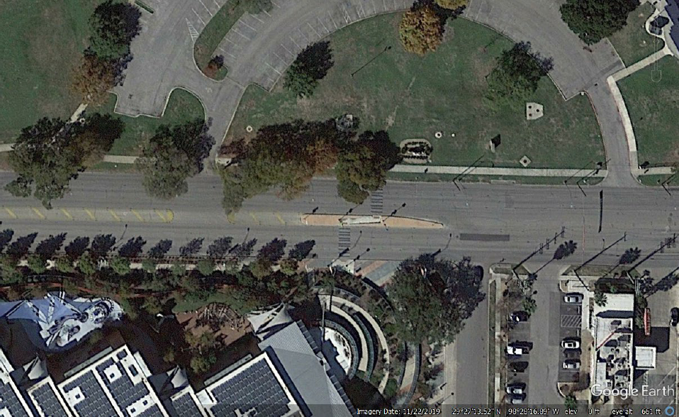
Source of base image: Google Earth (Google 2024)
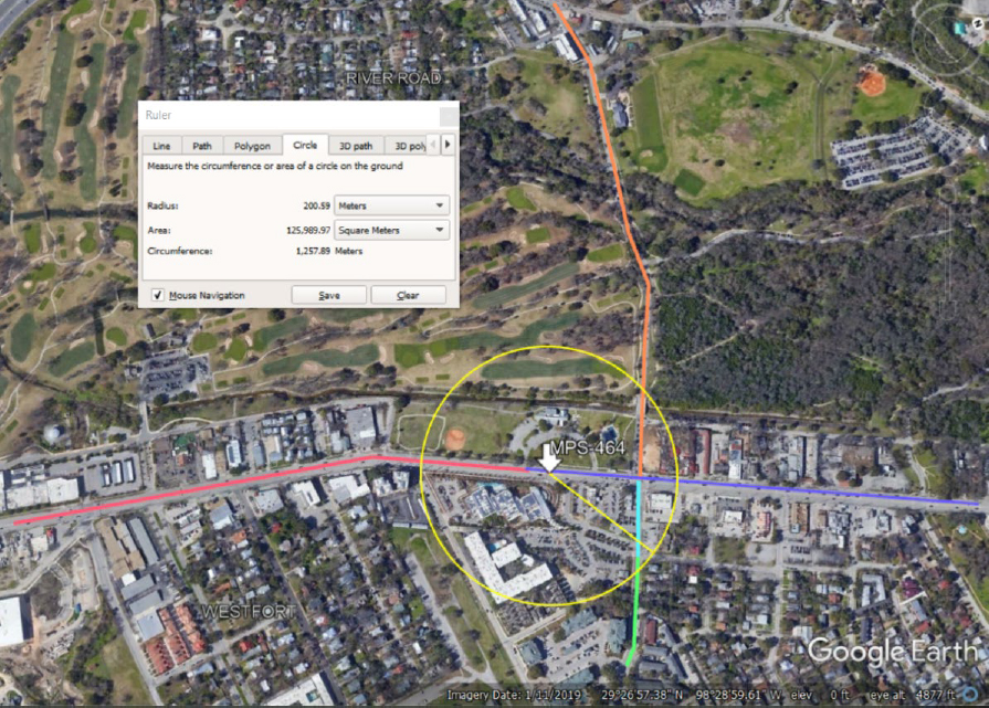
Source of base image: Google Earth (Google 2024)
Based on the factors described in Table D-32 and in the literature review, as well as parameters defined within the RFP and discussion with the project panel, the research team defined the following fixed variables to guide selection of study sites (also listed in Figure C-2):
- Posted speed limit: 30, 35, or 40 mph.
- Number of through lanes: 2 or 4.
- Horizontal alignment: tangent or minimal horizontal curve.
- Two-way roads only (i.e., no one-way roads).
In the first round of gathering data on road variables, the research team focused on the variables listed above, to determine which segments contain these variables of primary interest. In addition to the above selection criteria, the research team developed a list of criteria that were desirable for obtaining a sample of sites that represent a distribution of the factors of interest. While emphasizing the three posted speed limit values of 30, 35, and 40 mph and the criteria in Figure C-2, researchers also looked for sites with a variety of values in the following factors from Table D-32:
- Median type: raised, TWLTL, or none.
- Bike_1yes: bicycle lane presence.
- BldSet1to4: building setback category (1=no buildings within 100 ft, 2=buildings within 50-100 ft, 3=buildings within 20-50 ft, 4=buildings less than 20 ft).
- D1a: gross residential density (i.e., housing units per acre).
- D3a: total road network density (i.e., miles of roadway links per square mile).
These additional factors were chosen based on their discussion in the literature with all being related to contextual expectation effects on drivers for speeds that are appropriate or comfortable. Bicycle lanes are an indication of access and accommodation to non-motorized road users. Building setbacks affect the driver’s field of view and provides cues on context and vulnerable user presence. Residential density can suggest potential demand and the presence of a variety of road users, while road network density points to considerations such as the frequency of access points and the proximity of alternate routes. For the sites remaining in the database after the first round of road variables was collected, researchers conducted a second round of gathering the road variables listed in these four additional factors.
As discussed previously, researchers identified a variety of potential sources to identify study sites, including taking advantage of databases that were already in the possession of the research team. A summary of these potential sources is provided in Table D-34.
Table D-34. Summary of potential sources for Phase II study sites.
| Source | Data | State(s) | Comments |
|---|---|---|---|
| NCHRP Midblock Pedestrian Signals (Fitzpatrick et al. 2023) | Data for several factors for several study sites | CA, TX, UT | Dataset available from an ongoing NCHRP project that includes several factors of interest along with vehicle and pedestrian volume. Speed data need to be obtained. |
|
NCHRP 17-76 (Fitzpatrick et al. 2021b) TxDOT 0-7049 (Fitzpatrick et al. 2024) |
Data for several factors for several study sites | Texas | As part of Phase I activities, researchers built a large speed database for about 600 sites located in the City of Austin or within the San Antonio region. The City of Austin data are from the NCHRP 17-76 project on setting speed limits while the San Antonio region sites are from an ongoing TxDOT 0-7049 project. While the speed data in this database reflect binned data, the team used it to demonstrate the ability for non-free-flow speed data to identify relationships between operating speed and roadway, roadside, and other factors, see Chapter 6 for additional details. |
| FHWA PedCMF (Fitzpatrick et al. 2022) | Data for several factors for several study sites | OR, VA, WA | Dataset available from a recently completed FHWA project that includes several factors of interest along with vehicle and pedestrian volume. Speed data need to be obtained. |
| City of Dallas | Posted speed limits | Texas | Through a previous study, the research team mapped the posted speed limits for the Dallas area. The team identified the segments with 30-40 mph speed limits and identified the number of lanes and median type. Speed data need to be obtained. |
| City of Portland | Posted speed limits | Oregon | A database of traffic data available online from the City of Portland can be filtered on sites within the appropriate posted speed range (more than 300 sites with speed limits of 30-40 mph). Like the 17-76 data, the team can use the speed and volume data in the database, or simply use the list of sites to obtain speeds from big data sources and collect relevant site characteristics through in-office resources. |
| Online mapping | Posted speed limits | AZ, ME, MA, MI, MN, OH, UT, VA, WV | Road agencies of various states and cities maintain their own databases of roadway characteristics, which they provide online in the form of a mapping website. The roadway databases are searchable by speed limit. |
| Vendor data – HERE | Posted speed limits | All | Data used primarily for mapping applications can also be used as a resource for identifying study sites with desired speed limits and other characteristics of interest. Requires obtaining a license to access the data in the desired regions. |
The sources of previously collected data provided a set of almost 1800 study sites, as listed in Table D-35. Approximately half of those sites had a 30-mph speed limit (879 sites).
Table D-35. Summary of study sites contained in available databases.
| Source | PSL | CA | OR | TX | UT | VA | WA | Grand Total |
|---|---|---|---|---|---|---|---|---|
| 15-76_Test (17-76 & 7049) | 30 | 318 | 318 | |||||
| 15-76_Test (17-76 & 7049) | 35 | 87 | 87 | |||||
| 15-76_Test (17-76 & 7049) | 40 | 62 | 62 | |||||
| City of Portland online dataset | 30 | 172 | 172 | |||||
| City of Portland online dataset | 35 | 109 | 109 | |||||
| City of Portland online dataset | 40 | 67 | 67 | |||||
| City of Dallas (TxDOT study) | 30 | 46 | 46 | |||||
| City of Dallas (TxDOT study) | 35 | 104 | 104 | |||||
| City of Dallas (TxDOT study) | 40 | 84 | 84 | |||||
| MPS (NCHRP ongoing study) | 30 | 83 | 95 | 26 | 204 | |||
| MPS (NCHRP ongoing study) | 35 | 114 | 100 | 28 | 242 | |||
| MPS (NCHRP ongoing study) | 40 | 23 | 64 | 7 | 94 | |||
| PedCMF (FHWA study) | 30 | 82 | 6 | 51 | 139 | |||
| PedCMF (FHWA study) | 35 | 23 | 30 | 15 | 68 | |||
| PedCMF (FHWA study) | 40 | 1 | 1 | |||||
| Grand Total | 220 | 454 | 960 | 61 | 36 | 66 | 1797 |
In addition to the sites listed in Table D-35, researchers identified city and state jurisdictions that provide and maintain websites with online mapping tools and associated databases of roadway characteristics. These tools contained posted speed limit as a layer or filter that can be searched to identify roadway segments with potential for use as study sites. Cities contained in these online databases provide additional geographical distribution across the country and thousands of segments for consideration as study sites. The combination of the data already obtained and the online databases provided sources for sites in five regions of the country: northwest, southwest, south central, north central, and northeast. Researchers used a combination of these sources of data already acquired and additional available data to assemble a database of thousands of segments distributed nationwide.
The research team presented the previous information in the Interim Panel Meeting. At the direction of the project panel, the team also included Florida and Massachusetts in Phase II, in addition to the states identified in Phase I, to provide more geographical diversity in the study segments. The team initially identified tens of thousands of potential segments in each of those two states through ArcGIS roadway inventory files published by the respective state DOTs. Using those files, the team searched the INRIX XD™ segment database to determine which of those potential segments from the state DOT inventories had corresponding entries in INRIX XD™, which confirmed the existence of tens of thousands of potential segments. The team then obtained and matched speed data for segments from all of the considered states (i.e., California, Florida, Massachusetts, Oregon, Texas, Utah, Virginia, and Washington) from the INRIX XD™ speed database. The matching step was necessary because the team needed to confirm that a segment was present in the INRIX XD™ speed database and had available speed data. Because of the large number of segments in Florida and Massachusetts, the team decided to focus efforts on Miami-Dade County and Middlesex County in those two respective states to provide a more manageable set of segments and to not overwhelm the sample of segments from the other states.
Based on these efforts, the team identified several potential segments in California, Florida, Massachusetts, Oregon, Texas, Utah, Virginia, and Washington.
The research team further reviewed the list of potential factors provided in Table D-32 based on direction from the panel at the Interim Meeting. The team decided to proceed with a similar list of factors for analysis in Phase II, but they grouped the factors list based on similarities in data collection method. Details of each data collection round and their respective data collection methods are provided in Appendix F.


