Designing for Target Speed, Volume 1: Operating Speed and Road Elements (2026)
Chapter: Appendix F: Relationships Between Operating Speed and Road Elements on Roads with 25 to 40 mph Speed Limits
APPENDIX F. RELATIONSHIPS BETWEEN OPERATING SPEED AND ROAD ELEMENTS ON ROADS WITH 25 TO 40 MPH SPEED LIMITS
The central issue to achieving target speeds involves the configuration and operation of roadways so that target speeds, compatible with context and all roadway users, are chosen by—and not forced upon—vehicle operators (Fitzpatrick et al. 2021b, Fitzpatrick et al. 2021c). However, much of the roadway context, especially the urban one, has already been established, so a large part of the effort of achieving target speeds involves retrofitting the existing environment. Since only elements like lane widths, cross-sections including road diets, elements on the roadside such as street furniture or trees, and vertical and horizontal deflections are available to alter from a physical standpoint, a clear understanding of what factors help to achieve target speeds (or at least greatly influence operating speeds) is needed. To that end, the research team compiled information on segment locations and characteristics to develop a database for analysis, then conducted a series of analyses to determine the relationships between speed and the factors of interest.
DATA COLLECTION / BUILDING DATABASE
Segment Identification
Segment identification and selection began in Phase I with reviewing databases previously developed by members of the research team, as discussed in Appendix C and Appendix D. This approach permitted the team to have a larger database since some of the time-consuming data collection efforts were already done. Segments were available for California, Oregon, Texas, Utah, Virginia, and Washington from those sources. In Phase II, the research team selected additional segments from those states as well as segments from Miami-Dade County in Florida and Middlesex County in Massachusetts, as discussed in Appendix F.
INRIX Speed Data
INRIX compiles and aggregates crowdsourced, passively collected data from a variety of different sources and data resellers, including from smartphones, connected cars, fleet telematics, and fixed-sensor networks. They blend these data sources using proprietary algorithms to produce segment-based traffic speeds. Previously, INRIX focused on major highways and arterial streets. Recently, they added the INRIX XD™ traffic service, which includes non-freeways in many locations across the country. Speed data are compiled into a speed database that contains speed data for each individual segment aggregated by hour or by 15-minute period. The hourly file, commonly described as the “NAS168 File”, contains the collected speed data for each segment for each of the 168 hours of the week.
In the early activities of Phase II of NCHRP 15-76, the research team identified a variety of speed measures from probe speed data obtained from INRIX as having the potential to represent the operating speed that would have the best relationship with site characteristics. In some cases, the speed measure represented average conditions. In others, the research team attempted to identify speed measures that could represent free-flow conditions. These speed
measures were also considered in the context of whether they were as good as (or better than) spot speed measures at identifying site characteristics that are associated with operating speed at a site. Overall, several INRIX-based speed measures identified a similar number of (or more) variables as those identified for the at-site spot speed measures that used tube speed data, and researchers selected the ffspd variable from INRIX as the response variable for the analyses in this task. Details of the review, consideration, and selection of speed measures are provided in Appendix E.
The research team requested and received the NAS168 data file for calendar year 2019 to use in this effort. In addition to the hourly speed data, the NAS168 file also contains a variable named “ffspd”, an abbreviation for free-flow speed or reference speed. For the file from calendar year 2019, this value represents the 67th percentile observed speed for all time periods available in 2019. Other segment descriptors in the NAS168 file include the road or street name; the direction of travel; the starting and ending latitude and longitude for each segment; the location by state, county, and ZIP code; and the segment length.
Sources for Segment Characteristics
The research team believed that there are several roadway characteristics that can help explain typical operating speeds for a segment. The team identified variables of interest using their engineering knowledge along with findings from previous research studies. They also identified several existing databases that could provide these variables of interest. The sources used to generate segment characteristics include the following:
- Roadway characteristics data obtained from measurements made using aerial and street level photographs.
- EPA SLD provided several variables that described the characteristics of the areas around the roadway segment (US EPA 2025a).
- Building height was obtained from the United States Geological Survey (USGS) data catalog (Falcome 2016).
- Distance to buildings from the roadway center were obtained from U.S. Building Footprint dataset (Microsoft 2019).
- School presence was obtained from several sources as discussed below.
- Traffic volume and posted speed limit data obtained through online databases from state and local agencies.
For those databases with a shapefile, the research team used a GIS application to extract the data of interest that are linked to the roadway segments to build the database for the execution of this project. The team used the INRIX XD data to overlay and extract the SLD, building, school, traffic volume, and posted speed limit data. The next sections present additional information on how the database was assembled.
Roadway Characteristics Data
For those characteristics that had to be obtained using aerial or street views, the collection efforts were divided into “rounds” based on data collection method. In general, the rounds were as follows:
- Round 1 collected the presence of a feature, such as median type or sidewalk.
- Round 2 counted the number of driveways, unsignalized intersections, signalized intersections, and roundabouts.
- Round 3 measured the width for features of interest such as the width of the median or average lane width.
- Round 4 searched for the posted speed limit for the segment if not available from other sources.
- Round 5 gathered segment characteristics that required using both aerial and street view along with judgment on assigning a score.
- Round 6 used the Round 2 data to calculate the density of intersections by type.
The data for the rounds were collected via the aerial and street view mapping resources available in Google Earth and Google Maps. The research team used Google Earth’s historical views to obtain the 2019 aerial view and street view for that segment. If no image was available from 2019, researchers used images from earlier years. To aid in efficiency of data collection, segments that ran parallel to each other (i.e., opposite sides/directions of travel on the same street) were matched as a pair in the spreadsheet database, as data for both segments could be recorded at once.
Within each round of data collection, a “Keep or Drop” column in the database was used to keep track of segments that were dropped from the database for any reason to avoid data collection in future rounds for segments already identified to be removed. Comment columns in the database also provided a place for any notes or questions about a segment for later reference. There were many reasons for removing a segment that would be considered non-typical or outside the scope of this project. In general, the primary reasons a segment was removed from consideration included the following:
- Posted speed limit was not 25, 30, 35, or 40 mph.
- A posted speed limit could not be identified near the segment of interest or changed within the segment.
- One-way operation was present on the segment (the database only included segments with two-way operation).
- Segment length was less than 0.05 mile.
- Segment did not have either two through lanes or four through lanes consistently within the segment. For example, those segments with a total of three through lanes were removed. Segments were also removed if a through lane was added or dropped within the segment length.
- Segment was completely contained within a ramp or an auxiliary lane (e.g., a free-flow right-turn lane).
- Available images on Google Earth were during construction periods, preventing confirmation of critical site characteristics.
The following sections provide additional details on how these variables were collected within each round.
Round 1
Round 1 factors were characteristics that could be collected from Google Earth imagery, primarily through aerial views. The street views were only used at this stage if the data could not be gathered from the aerial view.
It was necessary to first identify if the segment had one-way operation or two-way. One-way segments were dropped from the database at this point. The number of through travel lanes in the segment, not including turning lanes, was recorded. For segments where the number of through lanes was greater than four, the segment was dropped from the database leaving only segments with 2 or 4 through lanes.
Sidewalk presence was recorded by entering 1 for sidewalk present on both sides of the street for the majority of the corridor, 0.5 for sidewalk present along one direction of travel for the majority of the corridor, 0 for no sidewalk present, or 99 for a mix (these segments were later reviewed). The sidewalk presence was later refined to represent the direction of travel and then combined with the presence or absence of a separation between the roadway and the sidewalk (see Sidewalk in Table for levels considered). Curb presence (“CurbGut_1yes”) was recorded in the same manner as sidewalk presence.
A general assessment of the horizontal alignment of the segment was noted in the “Horz_1tan” variable, where a value of 1 noted a relatively straight or tangent alignment and zero indicated at least one curve in the segment.
Bike lane presence in Round 1 was recorded by entering 1 for bike lane present along both sides of the street for the majority of the corridor, 0.5 for bike lane present along one side of the street for the majority of the corridor, 0 for no bike lane present, 8 if sharrows were present, or 99 for a mix (these segments were later reviewed). The presence of a bike lane was later refined to reflect the direction of travel and then combined with the type of separation between the bike lane and the travel lane (see BikeSepRev_DirOfTravel in Table for levels considered). Researchers used the same process for bike lane presence to note the presence of a parking lane (“Park_1yes”). A subsequent variable (“Park_DirOfTravel_1yes”, shown in Table) was developed to refine that information based on the direction of travel.
Median presence and type (“Median”) were recorded by entering None, Raised, TWLTL (for two-way left-turn lane), RR (for railroad tracks), or Other. Upon review, segments with a median entered as other included a few segments which were dropped, one which was identified as a raised median, and some which were “flush” medians. Researchers then noted the presence of center line markings (“CLmark”) and edge line markings (“ELmark”). The edge line markings variable was further refined based on direction of travel. Both of these marking variables are described in Table.
Table F-1 lists the variables used in the analysis that were based on those factors initially collected in Round 1.
| Variable | Description |
|---|---|
| BikeSepRev_DirOfTravel | Bicycle lane presence and type of separation between bike lane and motor vehicles: NoBikeLane (none or Sharrow) = no separated bike lane; PavementMarkingOnly = pavement marking is all that separates the bike lane from the motor vehicles; Buffer = space between vehicle and bike lane, but no vertical element; Vertical = some type of vertical element is present to separate bike lane from motor vehicle (includes curb) |
| CL_Mark | Center line marking presence: 0=no, 1=yes, median = median is present |
| CurbGut_DirOfTravel_1yes | Curb and gutter presence in direction of travel: 1=yes, 0=no, 90=mix (if condition is present/not present about 70% or more of segment then 1 or 0 is entered) |
| Elmark_DirOfTravel | Edge line marking presence in direction of travel: 0=no, 1=yes |
| Horz_1tan | Horizontal alignment: 1=straight(tangent), 0=some horizontal curvature (HC) |
| Median | Type of median: none, TWLTL, raised, RR, flush |
| NumLaneThruDir | Number of through lanes for the direction of travel (does not include TWLTL or turn lanes) |
| Park_DirOfTravel_1yes | On-street parking (either marked or unmarked) in direction of travel: 1=yes, 0=no, 90=mix (if condition is present/not present about 70% or more of segment then 1 or 0 is entered) |
| Sidewalk | Sidewalk presence: No sidewalk, Sidewalk with separation, Sidewalk without separation, or Sidewalk presence changes within segment |
Round 2
Round 2 factors were collected from Google Earth imagery, primarily through the aerial views. Segments that were dropped based on criteria from Round 1 data collection, as well as segments indicated as “Too Short” (i.e., segments less than 0.05 mile), were filtered out of the database prior to Round 2 data collection.
The direction of travel “DirTravel” for the study segment was recorded based on the bearing variable provided from INRIX data. The number of access points (i.e., non-single-family driveways and unsignalized intersections) along the XD segment in the same direction of travel and in the opposite direction of travel were counted. Figure F-1 provides an example of the counts for a sample segment. When a street is divided, the opposite-direction access points do not directly affect the vehicles traveling in the direction of travel. Instead, the median openings have an influence. Hence, on a divided street, only the number of access openings within the median were counted for the opposite direction of travel (see Figure F-2 for an example).
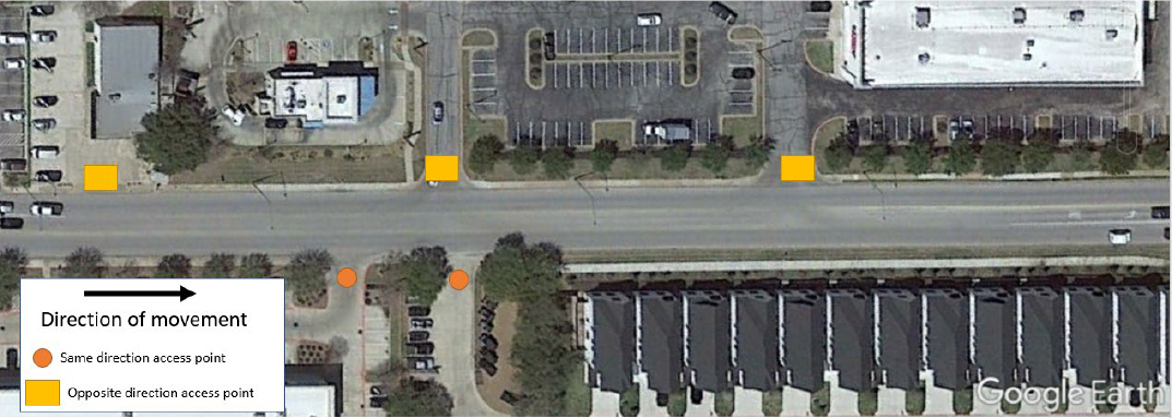
Source of base image: Google Earth (Google 2024)
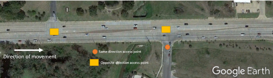
Source of base image: Google Earth (Google 2024)
The number of roundabouts within the XD segment, including at the limits of the segment, was counted as “RoundCount_XDSeg”. The number of signalized intersections (with either the typical traffic control signal or a pedestrian hybrid beacon) within the XD segment, including at the limits of the segment, was counted as “SignalCount_XDSeg”.
The type of intersections at the beginning (“IntCon_A”) and end (“IntCon_B”) of the XD segment were recorded as one of the following options:
- Sig = signalized intersection.
- Stop = stop control on the study segment (i.e., the vehicles on the segment need to come to a stop).
- Yield = yield control on the study segment.
- Round = roundabout intersection.
- Un = study segment is uncontrolled (e.g., two-way stop control for the intersecting street, no traffic control signal or PHB or all-way stop control).
- End = end of street (includes dead ends and cul-de-sacs).
- Mid = the segment ends at a midblock location (i.e., not at an intersection).
- 99 = some other condition (i.e., none of the above). Condition was described in the notes and later reviewed by senior members of the research team. The condition was either revised to one of the above categories or the segment was dropped.
These variables describing the intersection types at either end of the segment were combined into one variable (“INRIX-Seg_IntCon”), which does not specify direction of travel on the segment (i.e., assigning a beginning and end), but focuses on the various intersection types grouped by similar impact on operations. The entry options for this factor were the following:
- Sig&Sig = signalized intersections at both ends of segment
- Sig&StopEnd = one end of segment with signalized intersection and other end with stop control or end of street
- Sig&UnMidRou = one end of segment with signalized intersection and other end with uncontrolled intersection, at midblock, or roundabout
- Stop&StopEnd = one end of intersection with stop control and other end with stop control or end of street
- Stop&UnYieldEnd = one end of intersection with stop control and other end with uncontrolled intersection or yield control OR one end of segment with end of street and the other end with uncontrolled intersection
- UnMidRouYie&UnMidRouYie = uncontrolled intersection, at midblock, roundabout, or yield control at both ends of segment
Round 2 originally collected data for the entire XD segment length (which ranged between 0.05 and 1.00 mile); this had the potential to produce some extreme per-mile density values for some segments that might affect the influence of the factor in the analysis. Therefore, the research team decided to also define a 0.5-mile length centered on the midpoint of each XD segment and count the access points, roundabouts, and signals for those distances as well. The 0.5-mile length provided a consistent dimension for all study segments to compare, while providing a manageable length for data collection.
Round 2 also provided a chance to review Round 1 Roadway–Cross-Section characteristics as they pertained to the segments’ direction of travel, as well as “99” entries. The per-direction number of lanes, as well as per-direction presence of edge line markings, curb, parking lane, bicycle lane and separation, and sidewalk, based on the characteristics collected in Round 1, were documented here in Round 2. Some segments with zero through lanes (i.e., only exclusive turn lanes) in the direction of travel were identified at this point and dropped from the database.
See Table F-2 for the list of variables that originated in Round 2. The factors collected in this round were used for density calculations in Round 6.
Table F-2. Description of variables used in the analysis that were collected in Round 2 and Round 6.
| Variable | Description |
|---|---|
| DrvUsigPerMileBoth_0.5Mi | Driveways/unsignalized intersections per mile in both directions of the 0.5-mile segment divided by the 0.5-mile segment length |
| DrvUsigPerMileBoth_XDSeg | Driveways/unsignalized intersections per mile in both directions of the XD segment divided by the XD segment length |
| INRIX-Seg_IntCon | Type of intersection at both ends of XD segment: Sig&Sig = signals at both ends of the INRIX segment. Sig&StopEnd = signal on one end and stop or end of segment at other. Sig&UnMidRou = signal on one end and either Mid, Un, Roundabout, or Yield at the other. Stop&StopEnd = stop on one end and either stop or end on other. Stop&UnYieldEnd = stop on one end and either un or yield on other OR End on one end with uncontrol on other. UnMidRouYie&UnMidRouYie = either un, mid, round, or yield on both ends. |
| RoundPerMile_0.5MiSeg | Number of roundabout intersections along the 0.5-mi segment, including roundabouts located at the begin or end of the segment, divided by the length of segment in miles |
| RoundPerMile_XDSeg | Number of roundabout intersections along the Inrix XD segment, including roundabouts located at the begin or end of the segment, divided by the length of segment in miles |
| SigPerMile_0.5miSeg | Number of signalized intersections along the 0.5-mile segment, including any signals at the begin or end of the segment, divided by the length of segment in miles |
| SigPerMile_XDSeg | Number of signalized intersections along the Inrix XD segment, including any signals at the begin or end of the segment, divided by the length of segment in miles |
Round 3
Round 3 factors were collected from Google Earth aerial views, primarily measured using the “Ruler” tool. Measurements were rounded to the nearest whole foot and taken at the segment’s midpoint, unless the midpoint was located at an intersection, then measurements were collected at a location near the midpoint where the segment’s characteristics were more appropriately reflected.
For a segment in which a median was present, the median width (“MedWidth”) was measured and entered. When no median was present, 0 was entered. The total width of through lanes for the direction of travel (“TotalThruLaneWidth”) was measured from the center line of the street or the edge of the median to the edge line or outer edge of the travel lane(s). The average lane width (“AvgLaneWidth”) for the direction of travel was calculated by dividing the total width of through lanes by the number of through lanes in the direction of travel. Segments with lane width values less than 8 ft or greater than 20 ft were later reviewed. Some of these widths were due to changes in the number of lanes within the segment; in these cases, the segments were dropped. Other segments with larger widths had on-street parking that was not marked as a parking lane, so the travel lane, in absence of any parked vehicles, was wider than typical; these segments were retained for analysis. A review to correct entry errors for the
number of lanes, presence of on-street parking, or roadway cross-section type addressed other unusual through lane widths.
The bike lane width for the direction of travel (“BikeLnWidth”) was measured from the outer edge of the vehicle lanes or edge line to the outer edge of the bike lane. If a bike lane was not present, 0 was entered. The width of the shoulder for the direction of travel (“ShldWd”) was measured as the width between the edge line and the edge of pavement or between the edge line and the curb. Typically, if neither an edge line nor a curb was present, or if a curb was present but no edge line, the shoulder width was zero. If a bike lane was present, the shoulder measurement started from the outer edge of the bike lane.
The distance between roadway edges (“EdgeToEdge”) was measured at the midpoint for the segment from the outer edge of the right-most lane on the opposite direction of travel to the outer edge of the right-most lane on the same direction of travel. If bike lanes or parking lanes were present, they were included in the measurement. Segments with significantly larger edge to edge measurements were caused by divided roads.
The presence of a speed hump (“SpeedHump”) along the segment was recorded by entering 1, otherwise 0 was entered.
See Table F-3 for the list of variables in Round 3 that were ultimately used in the analysis.
| Variable | Description |
|---|---|
| AvgLaneWidth | Typical or average lane width for the segment (ft) |
| BikeLnWidth | If a bike lane is present, the width is measured as the distance from the outer edge of the vehicle lanes to the outer edge of the bike lane (ft) |
| EdgeToEdge | Distance between roadway edges at the midpoint for the segment (ft). The distance from the outer edge of the right-most lane on the opposite direction of travel to the outer edge of the right-most lane on the same direction of travel in the middle of the study segment. If bike lanes or parking lanes exist, they are included in the measurements. |
| MedWidth | Typical or average median width for the segment (ft) |
| ShldWd | Width of the shoulder (ft) for the direction of travel. The shoulder width is generally the width between the edge line and the edge of pavement or between the edge line and the curb. The shoulder width is zero if neither an edge line nor a curb is present. If a bike lane is present, the shoulder starts from the outer edge of the bike lane. |
| SpeedHump | Speed hump presence: 1=yes or 0=no |
Round 4
For the segments in which posted speed limits were not found in another database, the research team identified posted speed limits by “driving” along the segment in street view to find regulatory speed limit signs, (i.e., not school speed limit sign or a warning speed sign). Segments with a PSL less than 25 mph or greater than 40 mph were marked for dropping and additional data were not collected. If differing PSLs existed within one segment, the speed that applied to
most of its length was entered; segments in which the speed limit changed near the midpoint were dropped.
Round 5
Round 5 consisted of roadside characteristics collected from Google Earth utilizing both aerial and street view images. Table F-4 summarizes these variables.
| Round | Variable | Description |
|---|---|---|
| 4 | PSL | Posted speed limit (mph) |
| 5 | Fence1to3 | Fence characteristics, based on a 1-3 scale (1=no fence or minimal fencing, 2=Solid/privacy fence (e.g., wood, stone, brick) 10-20 ft from road, 3 = Fence within 10 ft of road) |
| 5 | StFurn1to4 | Street Furniture characteristics, based on a 1-4 scale (1=no street furniture, 2=Isolated street furniture greater than 20 ft from road, 3=Isolated street furniture within 20 ft, 4=Outside dining (tables and chairs), benches, and/or many objects next to edge of street) |
| 5 | StTree1to3 | Street Trees characteristics, based on a 1-3 scale (1=no trees within 30 ft or isolated/small tree, 2=A few trees but generally spaced about 30 ft apart and 20 ft from street edge, 3=Large tree and/or multiple trees within 10 ft of street) |
Round 6
Round 6 developed densities using data from Round 2 factors. Factors were calculated first from the counts along the XD segment, then from counts along the 0.5-mile segment. Including counts and calculations for 0.5-mile segments allowed for standardization across segments. Densities were determined for driveways and unsignalized intersections, roundabouts, and signalized intersections per mile. Table F-2 provides the resulting variables from Round 2 data used as a basis for Round 6.
Review of Variables Collected Using Google Earth Images
The database was divided by state for the duration of data collection to allow for the collection of multiple states’ data by different team members simultaneously. Quality control checks were performed following each round by checking several random segments for accuracy. Once data collection was completed the individual state files were combined into one database for general accuracy checks. Relationships between factors, as well as the use of pivot tables in the database spreadsheet, allowed for the identification of potential errors in data entry. When those errors were identified, the segments were reviewed by senior team members and corrected.
EPA Smart Location Database (SLD)
The SLD summarizes several different indicators (i.e., variables) associated with the built environment or the location. (US EPA 2025a) Several of the variables are based on census block groups (CBGs) or core-based statistical areas (CBSAs) in which the CBG resides. Other
variables use data from the American Community Survey (ACS). Indicators include density of development, diversity of land use, street network design, and access to destinations as well as various demographic and employment statistics. Indicators of particular interest for relating to speed include population, walkability index, street intersection density, and employment density.
The research team used GIS applications to associate the SLD data to the study segments. Using a spatial join function, the census block group characteristics of the SLD were joined to the corresponding study segments, and the variables in Table F-5 were extracted from each census block group. Only the census block groups intersected by the INRIX XD segment were considered. Since one INRIX XD segment can transverse across multiple census block groups, the extracted data was aggregated for those segments. The data aggregation depended on the variable type. For instance, for number-based variables such as population, workers, and road network, summation was used to aggregate the quantities. Averaging was used to obtain the aggregated quantities for the percentage/proportion-based variables, such as the percentage of low-wage workers and the percentage of the working population.
Table F-5 lists the SLD variables selected for the project database. Because of the large number of variables, the research team selected a subset of these variables for the detailed statistical analysis. First, the research team reviewed all variables and determined the variables unsuitable for analysis. This included variables with a large proportion of missing data, administrative-related variables, and variables used for flagging the data. The research team emphasized the selection of variables for use in the analysis based on suitability for influencing operating speed. In addition, the research team selected the National Walkability Index score and did not include those variables used in creating the National Walkability Index score (e.g., intersection density). Table F-6 lists the SLD variables that were chosen for the analysis.
Table F-5. SLD variable description
| Variable | Description | When Segment Spans More Than One CBG |
|---|---|---|
| CBSA_POP | Total population in core-based statistical area (CBSA) for the relevant census block group (CBG) | Summed |
| CBSA_WRK | Total number of workers that live in CBSA | Summed |
| CountHU | Housing units, 2018 | Summed |
| D1A | Gross residential density (HU/acre) on unprotected land | Summed |
| D3A | Total road network density | Summed |
| E_PctLowWa | Percentage of low-wage workers (LowWageWk) out of the total number of workers in a CBG (work location), 2018 | Averaged |
| HH | Households (occupied housing units), 2018 | Summed |
| NatWalkInd | National Walkability Index score for CBG | Averaged |
| P_WrkAge | Percent of population that is working-age, 2018 | Averaged |
| Pct_AO0 | Percent of zero-car households in CBG | Averaged |
| Pct_AO1 | Percent of one-car households in CBG | Averaged |
| Pct_AO2p | Percent of two-plus-car households in CBG | Averaged |
| R_HiWageWk | # of workers earning $3333/month or more (home location), 2018 | Summed |
| R_LowWageW | # of workers earning $1250/month or less (home location), 2018 | Summed |
| R_MedWageW | # of workers earning > $1250/month but < $3333/month (home location), 2018 | Summed |
| R_PCTLOWWA | % LowWageWk of total #workers in a CBG (home location), 2018 | Averaged |
| Workers | # of workers in CBG (home location), 2018 | Summed |
Table F-6. Description of SLD variables that were used in the final analysis
| Variable | Description |
|---|---|
| D3A | Total road network density |
| HH | Households (occupied housing units), 2010 |
| NatWalkInd | National Walkability Index score for CBG. |
| PCT_AO1 | Percent of one-car households in CBG |
| PCT_AO2P | Percent of two-plus-car households in CBG |
The National Walkability Index measures the relative walkability (ease of walking around) for every block group in the country. The index uses the following variables from the SLD (US EPA 2025a, US EPA 2025b, Ramsey and Bell 2014):
- Intersection density (SLD variable D3b): Higher intersection density is correlated with more walk trips. D3b summarizes total intersection density, weighted to reflect connectivity for pedestrian and bicycle travel. While intersection density is often used as an indicator of more walkable urban design, the source data provides no information regarding the presence or quality of sidewalks.
- Proximity to transit stops (SLD variable D4a): Distance from population center to nearest transit stop. Shorter distances correlate with more walk trips.
- Diversity of land uses:
-
- Employment mix (SLD variable D2b_E8MixA): The mix of employment types in a block group (the eight-tier classification summarizes employment into the following groups: retail, office, service, industrial, entertainment, education, healthcare, and public administration). Higher values correlate with more walk trips.
- Employment and household mix (SLD variable D2a_EpHHm): The mix of employment types and occupied housing. A block group with a diverse set of employment types (such as office, retail, and service) plus many occupied housing units will have a relatively high value. Higher values correlate with more walk trips.
The SLD documentation (US EPA 2025a) further explains how the National Walkability Index is calculated. Each block group was assigned four ranked scores, one for each of the variables above. To score block groups, the block groups were placed into 20 quantiles by variable value (quantiles are groupings with equal numbers of records), each containing 5 percent of the total block groups. The block groups were then assigned a rank from 1 to 20 depending upon their quantile position. A ranked score of 1 was assigned to the block groups with the lowest relative values influencing walking, and a ranked score of 20 was assigned to the block groups with the highest relative values influencing walking, with intermediate scores in between. To keep the National Walkability Index methodology as simple as possible while still incorporating the known impact of the built environment on walkability, the variables were weighted as follows: 1/3 to each of the three categories of street intersection density, land use mix, and proximity to transit. The land use mix category was subdivided into two to account for the two different techniques of measurement; employment mix and employment and household mix were each weighted by 1/6 (US EPA 2025a).
The block groups are assigned their final National Walkability Index scores on a scale of 1 to 20. The scores are categorized as follows:
- 1 – 5.75: Least walkable.
- 5.76 – 10.5: Below average walkable.
- 10.51 – 15.25: Above average walkable.
- 15.26 – 20: Most walkable.
U.S. Buildings Footprint
The details for building setbacks were obtained from the U.S. Building Footprint dataset (Microsoft 2019). The dataset consists of 129,591,852 computer-generated building footprints derived using computer vision algorithms on satellite imagery. In this task, the INRIX XD shapefile and building setback shapefile were used. It was assumed that the segments in INRIX XD shapefile represent the center line of the travel direction.
The research team wanted to obtain the distances from the center line to the buildings. To do so, buffers of 5 ft to 50 ft, with an increment of 5 ft, were created on the INRIX segments. Figure F-3 illustrates a segment with the 5-ft and 50-ft buffer shown. The number of buildings within each buffer distance was counted and associated with a given INRIX XD segment along with identifying the smallest buffer that included at least one building.

Source of base image: map data from OpenStreetMap, https://www.openstreetmap.org/copyright (OpenStreetMap 2025)
The variable used within the analysis, C_BuildingSetback, indicated the shortest distance to any building along the segment and included the following levels:
- 05 = at least one building is within 5 ft of the segment center line.
- 10 = at least one building is between 5 and 10 ft from the segment center line.
- 15 = at least one building is between 10 and 15 ft from the segment center line.
- 20 = at least one building is between 15 and 20 ft from the segment center line.
- 25 = at least one building is between 20 and 25 ft from the segment center line.
- 30 = at least one building is between 25 and 30 ft from the segment center line.
- 35 = at least one building is between 30 and 35 ft from the segment center line.
- 40 = at least one building is between 35 and 40 ft from the segment center line.
- 45 = at least one building is between 40 and 45 ft from the segment center line.
- 50 = at least one building is between 45 and 50 ft from the segment center line.
- 55 = no building is within 50 ft of the segment center line.
Table F-7 provides the distribution of distances to buildings by state for the segments included in this study. Overall, very few segments had a building within 15 ft of the segment center line. Table F-8 provides the distribution by posted speed limit. As expected, buildings are closer to the roadway segment center line for those roads with lower posted speed limits.
Table F-7. Distribution of C_BuildingSetback by state.
| C_BuildingSetback | CA | FL | MA | OR | TX | UT | VA | WA | Total |
|---|---|---|---|---|---|---|---|---|---|
| 05 | 1% | 0% | 0% | 0% | 1% | 1% | 1% | 0% | 0% |
| 10 | 0% | 0% | 1% | 1% | 0% | 0% | 1% | 0% | 0% |
| 15 | 2% | 0% | 3% | 1% | 1% | 1% | 1% | 1% | 1% |
| 20 | 5% | 2% | 8% | 6% | 3% | 0% | 9% | 0% | 5% |
| 25 | 10% | 4% | 14% | 11% | 6% | 2% | 10% | 2% | 8% |
| 30 | 19% | 8% | 19% | 22% | 11% | 5% | 16% | 3% | 14% |
| 35 | 17% | 12% | 16% | 19% | 13% | 5% | 12% | 10% | 14% |
| 40 | 19% | 12% | 12% | 14% | 14% | 12% | 14% | 11% | 13% |
| 45 | 9% | 12% | 10% | 12% | 11% | 11% | 8% | 15% | 11% |
| 50 | 7% | 10% | 5% | 6% | 10% | 5% | 7% | 16% | 8% |
| 55 | 12% | 40% | 12% | 10% | 31% | 58% | 21% | 42% | 26% |
| Grand Total | 100% | 100% | 100% | 100% | 100% | 100% | 100% | 100% | 100% |
Table F-8. Distribution of C BuildingSetback by PSL.
| C_BuildingSetback | 25 mph | 30 mph | 35 mph | 40 mph | Grand Total |
|---|---|---|---|---|---|
| 05 | 1% | 1% | 0% | 0% | 0% |
| 10 | 1% | 0% | 0% | 0% | 0% |
| 15 | 2% | 2% | 0% | 0% | 1% |
| 20 | 7% | 5% | 3% | 2% | 5% |
| 25 | 12% | 9% | 6% | 4% | 8% |
| 30 | 19% | 13% | 12% | 9% | 14% |
| 35 | 12% | 15% | 13% | 11% | 14% |
| 40 | 14% | 14% | 14% | 11% | 13% |
| 45 | 9% | 10% | 13% | 10% | 11% |
| 50 | 7% | 9% | 8% | 9% | 8% |
| 55 | 16% | 23% | 30% | 45% | 26% |
| Grand Total | 100% | 100% | 100% | 100% | 100% |
Building Height
The research team obtained building height data from the USGS data catalog (Falcome 2016). The dataset contains the average heights of the buildings by census block groups. This dataset is a categorical mapping of estimated mean building heights by census block group in shapefile format for the entire United States. The data were derived from the NASA Shuttle Radar Topography Mission, which collected “first return” (top of canopy and buildings) radar data at 30-m resolution in February 2000 aboard the Space Shuttle Endeavor. This dataset was processed to estimate building heights nationally and then aggregated to block group boundaries. The block groups were then categorized into six classes, ranging from “Low” to “Very High” (see Table F-9), based on the mean and standard deviation breakpoints of the data.
Table F-9. Building height categories and associated descriptions (Falcome 2016).
| Height category | Description |
|---|---|
| Low | Lowest category of building heights; primarily 1-2 story buildings |
| Low-Medium | 2nd lowest category; primarily 2-3 story buildings |
| Medium | 3rd lowest category; primarily 3-4 story buildings |
| Medium-High | 3rd highest category; primarily 3-6 story buildings |
| High | 2nd highest category: primarily 4-9 story buildings |
| Very High | Highest category of building heights; buildings average 10 stories or higher |
The research team merged the building height and the INRIX XD segments using GIS tools. First, the building height shapefile was mapped on the GIS application, then the INRIX XD shapefile was overlaid on the building height shapefile. Using a join function, the census blocks with building height data were joined to the corresponding INRIX XD segment, where a buffer of 50 ft was considered. The join performed was one-to-many, meaning one INRIX XD segment was joined to corresponding building heights from all census blocks that intersected with the segment. As a result, each INRIX XD segment had a number of corresponding building heights. For instance, segment 441645872 contained two building height categories (see Table F-10). For these INRIX XD segments that were associated with multiple building height census blocks, the research team identified the number of each category of building heights for the segment, a sample of which is shown in Table F-11. The research team then identified the highest building height category for the segment and used that information in the analysis. The variable used in the analysis, C_BuildingHeight, included the following levels:
- 1=Low (1-2 stories).
- 2=Low-Medium (2-3 stories).
- 3=Medium (3-4 stories).
- 4=Medium-High (3-6 stories).
- 5=High (4-9 stories).
- 6=Very High (10 stories or higher).
Table F-12 shows the distribution of building heights by state. The segments in Utah had the highest proportion of Very High buildings, followed by California. Taller buildings were associated with lower posted speed limits as shown in Table F-13.
Table F-10. A sample of joined building height data for a selected INRIX XD segment.
| RoadName | XDSegID | Height category | Height Description |
|---|---|---|---|
| South Pleasant Valley Road | 441645872 | Medium | Primarily 3-4 story buildings |
| South Pleasant Valley Road | 441645872 | Low-medium | Primarily 2-3 story buildings |
| South Pleasant Valley Road | 441645872 | Low-medium | Primarily 2-3 story buildings |
| South Pleasant Valley Road | 441645872 | Low-medium | Primarily 2-3 story buildings |
Table F-11. A sample of final building height database.
| XDSegID | BH_Low | BH_Low-Medium | BH_Medium | BH_Medium-High | BH_High | BH_Very High |
|---|---|---|---|---|---|---|
| 170326691 | 0 | 0 | 0 | 0 | 1 | 0 |
| 170335495 | 0 | 0 | 0 | 1 | 0 | 0 |
| 170390783 | 0 | 0 | 0 | 0 | 2 | 0 |
| 170581257 | 0 | 1 | 0 | 0 | 0 | 0 |
| 170598423 | 0 | 0 | 0 | 0 | 2 | 0 |
| 170606484 | 0 | 1 | 0 | 0 | 0 | 0 |
| 170615948 | 0 | 0 | 0 | 0 | 2 | 0 |
| 170620796 | 0 | 0 | 0 | 0 | 2 | 0 |
| 170624065 | 0 | 0 | 0 | 0 | 1 | 0 |
Table F-12. Distribution of C_BuildingHeight by state.
| C_BuildingHeight | CA | FL | MA | OR | TX | UT | VA | WA | Total |
|---|---|---|---|---|---|---|---|---|---|
| 1 | 0% | 1% | 0% | 0% | 0% | 0% | 0% | 0% | 0% |
| 2 | 3% | 15% | 14% | 5% | 21% | 5% | 31% | 16% | 15% |
| 3 | 9% | 20% | 46% | 70% | 53% | 24% | 28% | 64% | 39% |
| 4 | 19% | 22% | 24% | 20% | 14% | 26% | 14% | 14% | 19% |
| 5 | 52% | 31% | 15% | 3% | 9% | 15% | 28% | 6% | 21% |
| 6 | 17% | 12% | 1% | 1% | 2% | 29% | 0% | 0% | 6% |
| Grand Total | 100% | 100% | 100% | 100% | 100% | 100% | 100% | 100% | 100% |
Table F-13. Distribution of C_BuildingHeight by PSL.
| C_BuildingSetback | 25 mph | 30 mph | 35 mph | 40 mph | Grand Total |
|---|---|---|---|---|---|
| 1 | 0% | 0% | 0% | 0% | 0% |
| 2 | 14% | 13% | 18% | 19% | 15% |
| 3 | 29% | 40% | 46% | 40% | 39% |
| 4 | 15% | 22% | 17% | 20% | 19% |
| 5 | 30% | 21% | 15% | 20% | 21% |
| 6 | 12% | 5% | 4% | 2% | 6% |
| Grand Total | 100% | 100% | 100% | 100% | 100% |
Schools
Table F-14 presents the data sources for school datasets across the states and cities of interest. The school data contains the coordinates of each school in the study region. The research team wanted to extract the total number of schools within 0.5 mile of the INRIX XD segment. Similar to the building setback data, a 0.5-mile buffer on the INRIX XD segment was created and schools within the buffers were counted as illustrated in Figure F-4.
Table F-14. Data sources for schools.
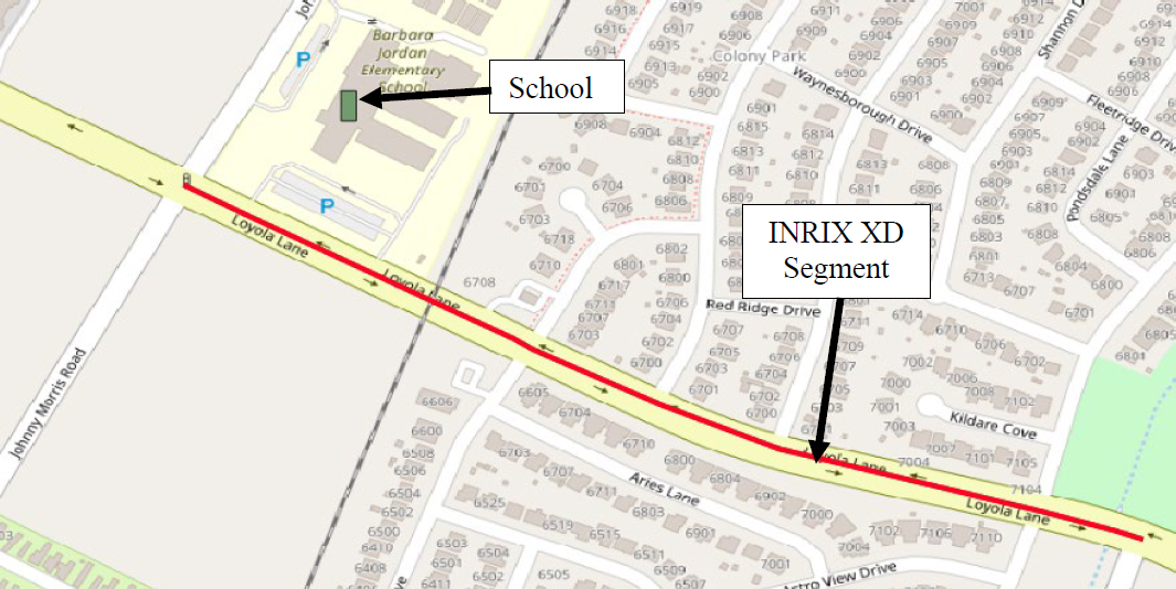
Source of base image: map data from OpenStreetMap, https://www.openstreetmap.org/copyright (OpenStreetMap 2025)
Traffic Volume and Posted Speed Limit
The research team obtained traffic volume and posted speed limit data from various sources, including previous projects and online state-based and nation-based databases. Table F-15 summarizes the sources used to obtain the data.
Table F-15. Data sources for traffic volumes and posted speed limits.
| State/City | Data Sources |
|---|---|
| California |
|
| Florida | |
| Massachusetts | |
| Oregon |
|
| Texas (Austin, Dallas, San Antonio) |
|
| Utah |
|
| Virginia | |
| Washington |
|
Similar to the external databases previously described, the research team used GIS tools to extract the posted speed limit and AADT associated with the INRIX XD segments. First, the INRIX XD shapefile of the segments was mapped in the GIS application. Using GIS tools, the coordinates of the midpoint of each INRIX XD segment were created and mapped. Using the midpoint coordinates, a buffer ranging between 15 ft and 50 ft, with an increment of 5 ft, was applied to associate the INRIX XD segments to the roadway characteristics shapefile. Varying buffers were applied to capture any possible misalignment between INRIX XD segment midpoints and the traffic volume and posted speed limit shapefiles. Using the “join” feature of the GIS application, the buffered midpoint of the INRIX XD segment was joined to the associated segment from various traffic volumes and posted speed limit shapefiles. After joining the two databases, the posted speed limit and AADT data were extracted.
Assembled Database for Analysis
The research team merged each of the datasets to the INRIX XD dataset. The objective was to confirm that each XD segment had its demographic data, building setback data, the associated number of schools, building height, and traffic data. The INRIX XD data acted as the base for the data integration, and all other data were overlayed on the INRIX XD data. The segments were mapped by direction of travel. Table F-16 presents the number of segments for each state and by each posted speed limit included in the final database.
Table F-16. Number of segments by state and posted speed limit.
| State | PSL = 25 mph | PSL = 30 mph | PSL = 35 mph | PSL = 40 mph | Total |
|---|---|---|---|---|---|
| California | 358 | 200 | 254 | 66 | 878 |
| Florida | 10 | 365 | 162 | 339 | 876 |
| Massachusetts | 165 | 683 | 361 | 137 | 1346 |
| Oregon | 128 | 165 | 27 | 7 | 327 |
| Texas | 88 | 788 | 419 | 153 | 1448 |
| Utah | 94 | 57 | 84 | 6 | 241 |
| Virginia | 391 | 44 | 211 | 2 | 648 |
| Washington | 150 | 255 | 140 | 18 | 563 |
| Total | 1384 | 2557 | 1658 | 728 | 6327 |
ANALYSIS
Variables and Summary Statistics
The assembled database included several variables that could affect speed. Based on preliminary investigations, variables were refined, combined, or eliminated for the eventual final evaluations. Table F-17 summarizes the variable descriptions for those variables considered in the final evaluations and Table F-18 provides the summary statistics. Most of the segments were two-lane undivided (3072 segments) or four-lane undivided (1220 segments). Other roadway types represented included two-lane divided (167 segments), two-lane with TWLTL (300 segments), four-lane divided (925 segments), or four-lane with TWLTL (643 segments).
Table F-17. Variable descriptions.
| Variable | Description |
|---|---|
| AADT | Average annual daily traffic (vehicles/day) |
| AvgLaneWidth | Average lane width for the direction of travel (ft) |
| BikeLnWidth | Distance between the edge line and the outer edge of the bike lane for the direction of travel (ft) |
| BikeSepRev_DirOfTravel | Type of separation between bike lane and motor vehicles: NoBikeLane (was N/A or Sharrow) = no separated bike lane. PavementMarkingOnly = pavement marking is all that separates the bike lane from the motor vehicles. Buffer = space between vehicle and bike lane, but no vertical element. Vertical = some type of vertical element is present to separate bike lane from motor vehicle (includes curb) |
| C_BuildingHeight | Code describing typical height of buildings: 1=Low (1-2 stories), 2=Low-Medium (2-3 stories), 3=Medium (3-4 stories), 4=Medium-High (3-6 stories), 5=High (4-9 stories), 6=Very High (10 stories or higher) |
| C_BuildingSetback | Code to reflect the offset distance between segment center line and nearest building: 05 = within 5 ft, 10 = between 5 and 10 ft, etc. |
| CenterTreat_1yes | Center line marking presence in the corridor: 0=no, 1=yes or median or TWLTL is present |
| CurbGut_DirOfTravel_1yes | Curb and gutter presence on segment for direction of travel: 1=yes, 0=no, 90=mix (if condition is present/not present about 70% or more of segment then 1 or 0 is entered) |
| Variable | Description |
|---|---|
| D3A | Total road network density, SLD variable |
| DrvUsigPerMileBoth_0.5Mi | Non-single-family driveways & unsignalized intersections per mile in both directions (access points / mile) |
| DrvUsigPerMileBoth_XDSeg | Non-single-family driveways & unsignalized intersections per mile in both directions (access points / mile) |
| EdgeToEdge | Distance between roadway edges at the midpoint for the segment (ft). |
| Elmark_DirOfTravel | Edge line marking presence in direction of travel: 0=no, 1=yes |
| Fence1to3 | Fence characteristics in direction of travel (based on a 1-3 scale): 1=no fence/minimal fencing/any fence that is not rating 2 or 3, 2=Solid/privacy fence (e.g., wood, stone, brick) 10-20 ft from road, 3 = Fence within 10 ft of road |
| Ffspd | Speed from Inrix XD representing the 67th percentile observed speed for all time periods available in 2019 |
| HH | Households (occupied housing units), 2018, SLD variable |
| Horz_1tan | Horizontal alignment with the in corridor: 1=straight/tangent (or relatively straight), 0=horizontal curvature (at least one curve near 90 degrees or multiple curves are present) |
| INRIX-Seg_IntCon | Description of intersection types at either end of the segment: Sig&Sig = signals at both ends of the INRIX segment. Sig&StopEnd = signal on one end and stop or end of segment at other. Sig&UnMidRou = signal on one end and either Mid, Un, Roundabout, or Yield at the other. Stop&StopEnd = stop on one end and either stop or end on other. Stop&UnYieldEnd = stop on one end and either un or yield on other OR End on one end with uncontrol on other. UnMidRouYie&UnMidRouYie = either un, mid, round, or yield on both ends. |
| Median | Type of median for the majority of the corridor: none, TWLTL, raised, RR, other |
| MedWidth | Median width for the segment at the midpoint (ft) |
| Miles | Length of INRIX XD segment in miles |
| NatWalkInd | National Walkability Index score for CBG. A measure of relative walkability at the block group level developed using variables in the SLD |
| NumLaneThruDir | Number of through lanes for the direction of travel (does not include TWLTL or turn lanes) |
| Park_DirOfTravel_1yes | On-street parking (either marked or unmarked) in direction of travel: 1=yes, 0=no, 90=mix (if condition is present/not present about 70% or more of segment then 1 or 0 is entered) |
| Pct_AO1 | Percent of one-car households in CBG, SLD variable |
| Pct_AO2p | Percent of two-plus-car households in CBG, SLD variable |
| PSL | The posted speed limit on the segment (mph) |
| R_HiWageWk | # of workers earning $3333/month or more (home location), 2018, SLD variable |
| R_LowWageW | # of workers earning $1250/month or less (home location), 2018, SLD variable |
| R_MedWageW | # of workers earning > $1250/month but < $3333/month (home location), 2018, SLD variable |
| R_PCTLOWWA | % LowWageWk of total #workers in a CBG (home location), 2018, SLD variable |
| Variable | Description |
|---|---|
| RoundPerMile_0.5MiSeg | Number of roundabout intersections along the 0.5-mi segment, including roundabouts located at the begin or end of the segment, divided by the length of segment in miles (roundabouts/mile) |
| RoundPerMile_XDSeg | Number of roundabout intersections along the Inrix XD segment, including roundabouts located at the begin or end of the segment, divided by the length of segment in miles (roundabouts/miles) |
| Schools_0.5mile | Number of schools within 0.5 mi of the segment |
| ShldWd | Width of the shoulder for the direction of travel (ft) |
| Sidewalk | Combining Sidewalk_DirOfTravel_1yes and SidewalkSep_DirOfTravel_1yes into one variable: No sidewalk, Sidewalk with separation, Sidewalk without separation, Sidewalk presence changes within segment |
| SigPerMile_0.5miSeg | Number of signalized intersections along the 0.5-mi segment, including any signals at the begin or end of the segment, divided by the length of segment in miles (signals/mile) |
| SigPerMile_XDSeg | Number of signalized intersections along the Inrix XD segment, including any signals at the begin or end of the segment (signals/mile) |
| SpeedHump | Is a speed hump present along the segment in year 2019? 1=yes or 0=no |
| State | State: California, Florida, Massachusetts, Oregon, Texas, Utah, Virginia, or Washington |
| StFurn1to4 | Street Furniture characteristics in direction of travel, based on a 1-4 scale: 1=no street furniture, 2=Isolated street furniture greater than 20 ft from road, 3=Isolated street furniture within 20 ft, 4=Outside dining (tables and chairs), benches, and/or many objects next to edge of street |
| StTree1to3 | Street Trees characteristics in direction of travel (based on a 1-3 scale): 1=no trees within 30 ft or isolated/small tree, 2=A few trees but generally spaced about 30 ft apart and 20 ft from street edge, 3=Large tree and/or multiple trees within 10 ft of street (including median) |
| Workers | # of workers in CBG (home location), 2018, SLD variable |
Table F-18. Summary statistics for variables used in the analysis (N=6327).
| Variable | Variable Type | Minimum | Maximum | Mean | Std. Dev. |
|---|---|---|---|---|---|
| AADT | Numerical | 350 | 59000 | 12604.8 1 | 10295.0 9 |
| AvgLaneWidth | Numerical | 8 | 23 | 12.66 | 2.98 |
| BikeLnWidth | Numerical | 0 | 16 | 0.95 | 2.31 |
| BikeSepRev_DirOfTravel | Categorical | Buffer (134), NoBikeLane (5292), PavementMarkingOnly (844), vertical (57) | |||
| C_BuildingHeight | Numerical | 1 | 6 | 3.63 | 1.15 |
| C_BuildingSetback | Numerical | 5 | 55 | 40.40 | 11.83 |
| CenterTreat_1yes | Categorical | 0 (418), 1 (5 | 09) | ||
| CurbGut_DirOfTravel_1yes | Categorical | 0 (649), 1 (5 | 56), 90 (22) | ||
| D3A | Numerical | 1.41 | 320.38 | 49.47 | 33.57 |
| DrvUsigPerMileBoth_0.5Mi | Numerical | 0 | 116 | 25.76 | 15.71 |
| DrvUsigPerMileBoth_XDSeg | Numerical | 0 | 154 | 29.25 | 21.69 |
| Variable | Variable Type | Minimum | Maximum | Mean | Std. Dev. |
|---|---|---|---|---|---|
| EdgeToEdge | Numerical | 16 | 122 | 46.28 | 18.82 |
| Elmark_DirOfTravel | Categorical | 0 (3457), 1 (2870) | |||
| Fence1to3 | Categorical | 1 (4407), 2 (501), 3 (1419) | |||
| ffspd | Numerical | 6 | 49 | 23.21 | 7.50 |
| HH | Numerical | 0 | 6384 | 1273.01 | 836.65 |
| Horz_1tan | Categorical | 0 (2125), 1 (4202) | |||
| INRIX-Seg_IntCon | Categorical | Sig&Sig (2199), Sig&StopEnd (281), Sig&UnMidRou (2056), Stop&StopEnd (109), Stop&UnYieldEnd (327), UnMidRouYie&UnMidRouYie (1355) | |||
| Median | Categorical | None (4257), Raised (1021), RR (64), TWLTL (955), Flush (30) | |||
| MedWidth | Numerical | 0 | 56 | 4.83 | 8.82 |
| Miles | Numerical | 0.05 | 1.00 | 0.32 | 0.26 |
| NatWalkInd | Numerical | 2.83 | 20.00 | 14.78 | 2.87 |
| NumLaneThruDir | Categorical | 1 (3550), 2 (2777) | |||
| Park_DirOfTravel_1yes | Categorical | 0 (4054), 1 (2262), 90 (11) | |||
| Pct_AO1 | Numerical | 0 | 0.85 | 0.40 | 0.13 |
| Pct_AO2p | Numerical | 0 | 0.95 | 0.47 | 0.20 |
| PSL | Numerical | 25 | 40 | 31.37 | 4.65 |
| R_HiWageWk | Numerical | 0 | 4221 | 728.06 | 539.35 |
| R_LowWageW | Numerical | 0 | 1717 | 312.80 | 214.73 |
| R_MedWageW | Numerical | 0 | 4254 | 444.68 | 355.68 |
| R_PCTLOWWA | Numerical | 0 | 0.48 | 0.21 | 0.06 |
| RoundPerMile_0.5MiSeg | Numerical | 0 | 6 | 0.04 | 0.37 |
| RoundPerMile_XDSeg | Numerical | 0 | 22 | 0.07 | 0.91 |
| Schools_0.5mile | Numerical | 0 | 13 | 1.76 | 1.94 |
| ShldWd | Numerical | 0 | 18 | 0.76 | 1.75 |
| Sidewalk | Categorical | No sidewalk (914), Sidewalk presence changes within segment (106), Sidewalk with separation (2098), Sidewalk without separation (3209) | |||
| SigPerMile_0.5miSeg | Numerical | 0 | 22 | 4.02 | 3.61 |
| SigPerMile_XDSeg | Numerical | 0 | 42 | 7.06 | 7.70 |
| SpeedHump | Categorical | 0 (6239), 1 (88) | |||
| State | Categorical | California (878), Floride (876), Massachusetts (1346), Oregon (327), Texas (1448), Utah (241), Virginia (648), Washington (563) | |||
| StFurn1to4 | Categorical | 1 (3040), 2 (116), 3 (2821), 4 (350) | |||
| StTree1to3 | Categorical | 1 (662), 2 (692), 3 (4973) | |||
| Workers | Numerical | 0 | 8539 | 1485.54 | 950.97 |
Analysis Approach
The research team utilized ffspd as a dependent variable (corresponding to a measure of operating speed) to explore the relationship between operating speed and various roadway, roadside, and non-roadway elements. The team employed ANCOVA models that included both categorical/discrete factors and continuous covariates as independent variables to explore the relationships between ffspd and many (50+) independent variables obtained from 6,327 segments. The ANCOVA models can be viewed as normal linear regression models and written as follows.
| yi = β0 + β1Xi1 +… + βK XiK + ei | (1) |
where a dependent variable yi represents operating speed (ffspd) at segment i, X1,…, XK are independent variables (various roadway, roadside, and non-roadway elements) that are either numerical or categorical (after converted to quantitative data through the use of some coding system such as dummy coding), β0, β1,…, βK are regression coefficients, and ei is an error term. Under the ANCOVA model, the interpretation of coefficients is straightforward and intuitive, and the estimated regression coefficients represent the effect sizes of independent variables associated with a unit change. The ANCOVA models have been extensively used to assess the effects of various independent variables on the dependent variable when the relationship between the independent variables and the response variable is deemed linear (as is or after applying appropriate transformations).
Table F-17 contains the list of all variables initially considered for the analysis, including operating speed, traffic volume, roadway characteristics, roadside characteristics, and relevant non-roadway features. Table F-18 provides the summary statistics. Note that not all potential independent variables in Table F-17 may have a significant relationship with a dependent variable. Also, some independent variables are highly correlated, which leads to the collinearity problem in parameter estimation if included simultaneously (Spiegelman et al. 2010). For example, corr(HH, CountHU)=0.9868, corr(Workers, R_LowWageW)=0.9006, and corr(R_LowWageW, R_MedWageW)=0.9161. Thus, the variables CountHU and R_LowWageW were excluded from the candidate predictors to prevent the collinearity problem.
Note that the response variable, ffspd, reflects the 67th percentile speed for the entire year and not the traditional 85th percentile speed (i.e., daytime only, free flow, etc.). Therefore, the results of these investigations should not be used for speed prediction; rather, the results provide an appreciation of what roadway characteristics may be influencing the speed the drivers are selecting on a given roadway segment.
FINDINGS
Several combinations of variables were explored during model development. The research team decided to focus on variables within the following five situations:
- Evaluation using only the posted speed limit variable. This evaluation could provide insight into the influence of the number on the speed limit sign.
- Evaluation using variables influenced by transportation professionals. This evaluati included variables that could be under the influence of a transportation professional.
- Evaluation using all available variables including demographics variables. This evaluation included any available variable that could help to identify conditions that are associated with different operating speeds.
- Evaluation focusing on average lane width. This evaluation explored the relationship between lane width and operating speed. Because initial efforts determined that average lane width was not significant, more focused subsets of the database were created in order to explore the potential relationship for segments with average lane width between 8 and 13 ft.
- Evaluation focusing on center line and edge line markings. This evaluation focused on the presence or absence of center line or edge line markings on the subset of the database containing two-lane roads with no median, an average lane width of no more than 13 ft, no mix of curbs and shoulders within the segment, and a PSL of 25 to 35 mph.
In the following models, the response variable was ffspd and state was included as a random effect. Based on preliminary results, the research team decided to use the number of driveways/unsignalized intersections, signalized intersections, and roundabout densities calculated based on 0.5-mile segments rather than the INRIX XD segment length, which ranged from 0.05 to 1 mile in length. Using the same segment length provides consistency in considering the portion of the road length that may be influencing a driver’s speed choice. Models that used both density values were explored, because the difference in INRIX XD segment lengths could give quite different density values; however, these models were determined to not be as good as the models that only used the 0.5-mile segment for calculating signal density, roundabout density, and DrvUsigPerMileBoth density (sometimes called access density).
Because of counterintuitive results, the following variables were removed from the final ANCOVA model that was based on all data:
- AvgLaneWidth (was explored using subset of the data, see Appendix G).
- StTree1to3.
- Horz_1tan.
Posted Speed Limit Evaluation
Table F-19 describes the overall fit of the model for the analysis that used only the posted speed limit variable, and Table F-20 details the parameter estimates for the selected model. In general, posted speed limit explains about 30 percent of the variability in operating speed for the 6,327 segments included in the database.
Table F-19. Summary of fit for analysis using posted speed limit variable only
| Measure | Value |
|---|---|
| RSquare | 0.306355 |
| RSquare Adj | 0.306245 |
| Root Mean Square Error | 6.253475 |
| Mean of Response | 23.21385 |
| Observations (or Sum Wgts) | 6327 |
Table F-20. Parameter estimates for analysis using posted speed limit variable only (N=6327).
| Term | Estimate | Std Error | DFDen | t Ratio | Prob>|t| |
|---|---|---|---|---|---|
| Intercept | 2.7439738 | 1.009893 | 14.91 | 2.72 | 0.0160* |
| PSL | 0.6457371 | 0.018334 | 6323 | 35.22 | <.0001* |
Transportation Professional Evaluation
Table F-21 details the estimates for the individual levels within each variable for the analysis that considered the variables that could be influenced by transportation professionals while Table F-22 shows the fixed effects results by variable. Most variables in the model were significant at the 0.05 level.
| Effect | Level | Estimate | Standard Error | DF | t Value | Pr > |t| |
|---|---|---|---|---|---|---|
| Intercept | Not applicable | 28.6192 | 0.9075 | 142 | 31.53 | <.0001 |
| AADT | Not applicable | 0.000054 | 7.16E-06 | 6260 | 7.6 | <.0001 |
| BikeLnWidth | Not applicable | 0.1516 | 0.08957 | 6288 | 1.69 | 0.0907 |
| BikeSepRev_DirOfTrav | Buffer | -0.5784 | 0.8478 | 6288 | -0.68 | 0.4951 |
| BikeSepRev_DirOfTrav | NoBikeLane | 0 | . | . | . | . |
| BikeSepRev_DirOfTrav | Pavement Marking Only | 0.4022 | 0.5034 | 6287 | 0.8 | 0.4243 |
| BikeSepRev_DirOfTrav | Vertical | 1.6729 | 0.9937 | 6287 | 1.68 | 0.0923 |
| C_BuildingHeight | Not applicable | -1.0286 | 0.07517 | 6026 | -13.68 | <.0001 |
| C_BuildingSetback | Not applicable | 0.04873 | 0.006142 | 6282 | 7.93 | <.0001 |
| CurbGut_DirOfTravel_ | 0 | 1.868 | 0.2434 | 6292 | 7.68 | <.0001 |
| CurbGut_DirOfTravel_ | 1 | 0 | . | . | . | . |
| CurbGut_DirOfTravel_ | 90 | 3.4554 | 1.0037 | 6285 | 3.44 | 0.0006 |
| D3A | Not applicable | 0.007717 | 0.002033 | 6292 | 3.8 | 0.0001 |
| DrvUsigPerMileBoth_0.5 Mi | Not applicable | -0.03536 | 0.004379 | 6263 | -8.08 | <.0001 |
| EdgeToEdge | Not applicable | 0.0054 | 0.006922 | 6291 | 0.78 | 0.4354 |
| Fence1to3 | 1 | 0 | . | . | . | . |
| Fence1to3 | 2 | 1.2265 | 0.2209 | 6290 | 5.55 | <.0001 |
| Fence1to3 | 3 | 0.4424 | 0.1512 | 6285 | 2.93 | 0.0034 |
| Median | Flush | -0.2782 | 0.8401 | 6286 | -0.33 | 0.7405 |
| Median | None | 0 | . | . | . | . |
| Median | Raised | -0.09161 | 0.2437 | 6291 | -0.38 | 0.707 |
| Effect | Level | Estimate | Standard Error | DF | t Value | Pr > |t| |
|---|---|---|---|---|---|---|
| Median | RR | -0.8066 | 0.6783 | 6265 | -1.19 | 0.2344 |
| Median | TWLTL | 0.7651 | 0.2023 | 6281 | 3.78 | 0.0002 |
| NatWalkInd | Not applicable | -0.4774 | 0.02696 | 6292 | -17.71 | <.0001 |
| NumLaneThruDir | 1 | -3.445 | 0.207 | 6292 | -16.64 | <.0001 |
| NumLaneThruDir | 2 | 0 | . | . | . | . |
| Park_DirOfTravel_1yes | 0 | 0 | . | . | . | . |
| Park_DirOfTravel_1yes | 1 | -0.5437 | 0.1634 | 6216 | -3.33 | 0.0009 |
| Park_DirOfTravel_1yes | 90 | -2.939 | 1.3788 | 6286 | -2.13 | 0.0331 |
| PSL | Not applicable | 0.2253 | 0.0155 | 6276 | 14.53 | <.0001 |
| RoundPerMile_0_5MiSeg | Not applicable | -0.2305 | 0.1581 | 6287 | -1.46 | 0.1448 |
| Schools_0_5mile | Not applicable | -0.04387 | 0.0367 | 6035 | -1.2 | 0.232 |
| ShldWd | Not applicable | 0.3121 | 0.03772 | 6292 | 8.27 | <.0001 |
| Sidewalk | No sidewalk | 0 | . | . | . | . |
| Sidewalk | Sidewalk presence changes within segment | -0.7073 | 0.4823 | 6286 | -1.47 | 0.1426 |
| Sidewalk | Sidewalk with separation | -0.2007 | 0.2172 | 6292 | -0.92 | 0.3554 |
| Sidewalk | Sidewalk without separation | -0.8406 | 0.2201 | 6289 | -3.82 | 0.0001 |
| SigPerMile_0_5miSeg | Not applicable | -0.6863 | 0.02253 | 6290 | -30.46 | <.0001 |
| SpeedHump | 0 | 0 | . | . | . | . |
| SpeedHump | 1 | -3.5662 | 0.5009 | 6289 | -7.12 | <.0001 |
| StFurn1to4 | 1 | 0 | . | . | . | . |
| StFurn1to4 | 2 | -0.329 | 0.4355 | 6290 | -0.76 | 0.4501 |
| StFurn1to4 | 3 | 0.9845 | 0.1291 | 6289 | 7.63 | <.0001 |
| StFurn1to4 | 4 | 0.5021 | 0.2792 | 6279 | 1.8 | 0.0721 |
| Effect | Num DF | Den DF | F Value | Pr > F |
|---|---|---|---|---|
| AADT | 1 | 6260 | 57.75 | <.0001 |
| BikeLnWidth | 1 | 6288 | 2.86 | 0.0907 |
| BikeSepRev_DirOfTrav | 3 | 6290 | 3.81 | 0.0097 |
| C_BuildingHeight | 1 | 6026 | 187.24 | <.0001 |
| C_BuildingSetback | 1 | 6282 | 62.94 | <.0001 |
| CurbGut_DirOfTravel_ | 2 | 6290 | 33.40 | <.0001 |
| D3A | 1 | 6292 | 14.41 | 0.0001 |
| DrvUsigPerMileBoth_0.5Mi | 1 | 6263 | 65.21 | <.0001 |
| EdgeToEdge | 1 | 6291 | 0.61 | 0.4354 |
| Fence1to3 | 2 | 6289 | 17.31 | <.0001 |
| Median | 4 | 6263 | 5.53 | 0.0002 |
| NatWalkInd | 1 | 6292 | 313.63 | <.0001 |
| NumLaneThruDir | 1 | 6292 | 276.98 | <.0001 |
| Park_DirOfTravel_1yes | 2 | 6265 | 7.49 | 0.0006 |
| PSL | 1 | 6276 | 211.24 | <.0001 |
| RoundPerMile_0_5MiSeg | 1 | 6287 | 2.13 | 0.1448 |
| Schools_0_5mile | 1 | 6035 | 1.43 | 0.2320 |
| ShldWd | 1 | 6292 | 68.45 | <.0001 |
| Sidewalk | 3 | 6289 | 9.01 | <.0001 |
| SigPerMile_0_5miSeg | 1 | 6290 | 927.52 | <.0001 |
| SpeedHump | 1 | 6289 | 50.69 | <.0001 |
| StFurn1to4 | 3 | 6283 | 20.50 | <.0001 |
Notable findings by variable include the following:
- AADT. Speeds were faster on streets with higher volume. For the range of AADT values present in this database (350 to 59000 veh/day), the speed change between the lowest and highest volumes was 3.2 mph.
- BikeLnWidth. The model indicated that speeds are faster on roads with wider bike lanes. The speed change estimated for a street with a 6-ft bike lane as compared to the widest bike lane in this database (16 ft) would be 1.5 mph.
- BikeSepRev_DirOfTrav. Speeds were lower by less than 0.6 mph when the bike lane was separated with a buffer and no vertical element as compared to segments with no bike lanes. Speeds were higher by less than 0.4 mph when the bike lane was separated with pavement markings only as compared to segments with no bike lanes. Speeds were higher by 1.7 mph when the bike lane was separated with a vertical element as compared to segments with no bike lane.
- C_BuildingHeight. Speeds were lower with increasing heights of buildings. This variable was one of the most influential variables in the models. The segments with the tallest buildings were estimated to have speeds that were 5.1 mph slower.
- C_BuildingSetback. Speeds were higher with increasing setback of buildings. The segments with buildings within a few feet had operating speeds that were estimated to be 2.5 mph slower.
- CurbGut_DirOfTravel. When curbs were not present (i.e., shoulders are present), speeds were higher (by about 1.9 mph). This finding is intuitive. A non-intuitive
- finding was that when there were changes between shoulders and curbs within the segment, speeds were 3.5 mph higher. This result may have been due to a small sample size; only 22 out of the 6,327 segments in the database had changes in curbs.
- D3A. This variable reflects the number of miles of road within the census block group area. In theory, having more roads within a set area should reflect a denser urban area which could be associated with lower speed. For the transportation professional model, this variable indicated that speeds are slightly faster with greater density. The speed difference between the smallest and largest values in the database was 2.5 mph.
- DrvUsigPerMileBoth_0.5Mi. More driveways are associated with slower speeds, as anticipated. For the range of access points present in this database (0 to 116 driveways or unsignalized intersections per mile), the speed difference is 4.1 mph slower for the segments with 116 access points per mile compared to no access points.
- EdgeToEdge. The wider the road the higher the speeds, but the difference was small (less than 0.6 mph between a road that was 16 ft wide compared to a road that was 122 ft wide). In addition, this variable was not statistically significant.
- Fence1to3. Higher speeds were identified when fences were within 10 to 20 ft from the road (1.2 mph) or within 10 ft of the road (0.4 mph) as compared to no or minimal fences.
- Median. A flush median was associated with slightly slower speeds (approximately 0.28 mph) as compared to the roads with no median. The results of this analysis found a near-zero (0.09 mph) speed difference between raised medians and none. Segments with RR in the median had lower speeds (by 0.81 mph) as compared to no median. This result was expected because the segments with a RR median type have light rail, which typically occurs on segments with lower PSL and in more dense urban areas. The presence of a TWLTL could be associated with greater separation between travel lanes, which could be associated with higher speeds. The TWLTL can result in more frequent conflicts, which could be associated with lower operating speed. For this database and model, speeds were found to be about 0.77 mph higher for sites with TWLTL as compared to segments with no medians.
- NatWalkInd. This variable has potential values of 1 to 20 possible, with 1= block groups with the lowest relative values influencing walking and a score of 20 for those block groups with the highest relative values influencing walking. The score considers intersection density, proximity to transit stops, employment mix, and employment and household mix. For this database, the range of values was 2.83 to 20.0. The segments with a value of 20 would have operating speeds that are about 8.2 mph lower as compared to those segments with a NatWalkInd of 2.83.
- NumLaneThruDir. Speeds were found to be slower on 2-lane roads as compared to 4-lane roads by 3.4 mph.
- Park_DirOfTravel_1yes. Speeds were slower when on-street parking is present by 0.5 mph. Speeds were found to be even slower when there was a mix of on-street and no on-street parking, by 2.9 mph as compared to no on-street parking.
- PSL. Speeds were higher with increasing posted speed limit values. While influential, the speed change between the different speed limits was not as great as the posted speed limit increase. For example, a 5-mph increase in the posted speed limit (e.g.,
- from 30 to 35 mph) was associated with only about a 1.1 mph difference in operatin speed for the segments included in this database.
- RoundPerMile_0_5MiSeg. Speeds were slower when there were more roundabouts within the segment. For the range of RoundPerMile_0_5MiSeg values present in this database (0 to 6 roundabouts/mile), the speed change was 1.4 mph. However, this variable was not statistically significant.
- Schools_0.5mile. Speeds were slower when there are more schools in the area; however, the decrease was by only a small amount and the finding was not significant. The average value of the variable was about 2 schools in the 0.5-mile buffer, resulting in about 0.08 mph decrease in operating speed between no school and 2 schools within the 0.5-mile buffer.
- ShldWd. Speeds were higher with increasing shoulder width. For the range of shoulder width values present in this database (0 to 18 ft), the speed change is 5.6 mph.
- Sidewalk. Speeds were slower on streets where sidewalk presence changes within the segment, by 0.7 mph as compared to segments with no sidewalks. Speeds on streets with separated sidewalks were similar to the speeds on streets without sidewalks (0.2 mph). Speeds were slower on streets with sidewalks that do not have separation, by 0.8 mph as compared to segments with no sidewalks.
- SigPerMile_0_5miSeg. Speeds were lower with increasing number of signals on the segment. Of the intersection density variables, the signalized intersection variable was the most influential. This variable ranged between 0 and 22 signals per mile with an associated difference of 15.1 mph between the minimum and maximum signal densities. As a reminder, this variable was calculated based on the number of signals within 0.5 mile, adjusted to reflect signals per mile. Therefore, the segment with 22 signals per mile had 11 signals within a 0.5-mile section, or a signal every 240 ft.
- SpeedHump. Speeds were slower, by about 3.6 mph, when a speed hump was present on the segment.
- StFurn1to4. When compared to the condition of no street furniture, the segments with isolated street furniture greater than 20 ft from the road were associated with 0.3 mph slower speeds, the condition of isolated street furniture within 20 ft was associated with 1.0 mph faster speeds, and the condition of outside dining (tables and chairs), benches, and/or many objects next to edge of street was associated with 0.5 mph faster speeds. The expectation was that having more street furniture closer to the edge of the travel way would be associated with slower speeds. The research team does not have a theory as to why speeds were found to be faster when street furniture was observed as being within 20 ft of the roadway.
Demographics and Transportation Professional Evaluation
This section presents the analysis results that considered all variables included in the database described in the previous section. Table F-23 details the estimates for the individual levels within each variable while Table F-24 shows the fixed effects results by variable. Most remaining variables in the model were significant at the 0.1 level.
| Effect | Level | Estimate | Standard Error | DF | t Value | Pr > |t| |
|---|---|---|---|---|---|---|
| Intercept | Not applicable | 23.8397 | 1.0287 | 267 | 23.17 | <.0001 |
| AADT | Not applicable | 0.000049 | 7.10E-06 | 6255 | 6.95 | <.0001 |
| BikeLnWidth | Not applicable | 0.1694 | 0.08866 | 6285 | 1.91 | 0.0561 |
| BikeSepRev_DirOfTrav | Buffer | -0.5751 | 0.8389 | 6285 | -0.69 | 0.493 |
| BikeSepRev_DirOfTrav | NoBikeLane | 0 | . | . | . | . |
| BikeSepRev_DirOfTrav | Pavement Marking Only | 0.3547 | 0.4982 | 6284 | 0.71 | 0.4765 |
| BikeSepRev_DirOfTrav | Vertical | 0.9948 | 0.9848 | 6284 | 1.01 | 0.3125 |
| C_BuildingHeight | Not applicable | -0.737 | 0.07927 | 5948 | -9.3 | <.0001 |
| C_BuildingSetback | Not applicable | 0.04744 | 0.006088 | 6276 | 7.79 | <.0001 |
| CurbGut_DirOfTravel_ | 0 | 1.7569 | 0.2411 | 6289 | 7.29 | <.0001 |
| CurbGut_DirOfTravel_ | 1 | 0 | . | . | . | . |
| CurbGut_DirOfTravel_ | 90 | 3.275 | 0.9932 | 6282 | 3.3 | 0.001 |
| D3A | Not applicable | -0.00075 | 0.002428 | 6289 | -0.31 | 0.7575 |
| DrvUsigPerMileBoth_0.5Mi | Not applicable | -0.03099 | 0.004376 | 6260 | -7.08 | <.0001 |
| EdgeToEdge | Not applicable | 0.007343 | 0.006855 | 6288 | 1.07 | 0.2841 |
| Fence1to3 | 1 | 0 | . | . | . | . |
| Fence1to3 | 2 | 1.0855 | 0.219 | 6288 | 4.96 | <.0001 |
| Fence1to3 | 3 | 0.4379 | 0.1499 | 6281 | 2.92 | 0.0035 |
| HH | Not applicable | 0.000477 | 0.000089 | 6289 | 5.39 | <.0001 |
| Median | Flush | -0.1913 | 0.8314 | 6283 | -0.23 | 0.818 |
| Median | None | 0 | . | . | . | . |
| Median | Raised | -0.05159 | 0.2413 | 6288 | -0.21 | 0.8307 |
| Median | RR | -0.6414 | 0.6714 | 6257 | -0.96 | 0.3395 |
| Median | TWLTL | 0.6617 | 0.2007 | 6278 | 3.3 | 0.001 |
| NatWalkInd | Not applicable | -0.3955 | 0.02788 | 6289 | -14.19 | <.0001 |
| NumLaneThruDir | 1 | -3.4297 | 0.2052 | 6289 | -16.72 | <.0001 |
| NumLaneThruDir | 2 | 0 | . | . | . | . |
| Park_DirOfTravel_1yes | 0 | 0 | . | . | . | . |
| Park_DirOfTravel_1yes | 1 | -0.5457 | 0.1618 | 6199 | -3.37 | 0.0007 |
| Park_DirOfTravel_1yes | 90 | -2.9921 | 1.3642 | 6283 | -2.19 | 0.0283 |
| Pct_AO1 | Not applicable | 0.05908 | 0.6541 | 6289 | 0.09 | 0.928 |
| Pct_AO2p | Not applicable | 4.5766 | 0.5085 | 6288 | 9 | <.0001 |
| PSL | Not applicable | 0.2216 | 0.01535 | 6266 | 14.43 | <.0001 |
| RoundPerMile_0_5MiSeg | Not applicable | -0.2532 | 0.1565 | 6284 | -1.62 | 0.1057 |
| Schools_0_5mile | Not applicable | 0.0043 | 0.03668 | 6009 | 0.12 | 0.9067 |
| ShldWd | Not applicable | 0.3023 | 0.03741 | 6289 | 8.08 | <.0001 |
| Sidewalk | No sidewalk | 0 | . | . | . | . |
| Sidewalk | Sidewalk presence changes within segment | -0.8132 | 0.4774 | 6283 | -1.7 | 0.0885 |
| Sidewalk | Sidewalk with separation | -0.2605 | 0.2151 | 6289 | -1.21 | 0.2258 |
| Sidewalk | Sidewalk without separation | -0.8024 | 0.2179 | 6286 | -3.68 | 0.0002 |
| Effect | Level | Estimate | Standard Error | DF | t Value | Pr > |t| |
|---|---|---|---|---|---|---|
| SigPerMile_0_5miSeg | Not applicable | -0.6551 | 0.02252 | 6287 | -29.09 | <.0001 |
| SpeedHump | 0 | 0 | . | . | . | . |
| SpeedHump | 1 | -3.6472 | 0.4956 | 6286 | -7.36 | <.0001 |
| StFurn1to4 | 1 | 0 | . | . | . | . |
| StFurn1to4 | 2 | -0.4299 | 0.431 | 6287 | -1 | 0.3186 |
| StFurn1to4 | 3 | 0.8988 | 0.1283 | 6283 | 7.01 | <.0001 |
| StFurn1to4 | 4 | 0.4972 | 0.2771 | 6275 | 1.79 | 0.0728 |
| Effect | Num DF | Den DF | F Value | Pr > F |
|---|---|---|---|---|
| AADT | 1 | 6255 | 48.28 | <.0001 |
| Median | 4 | 6258 | 4.03 | 0.0029 |
| NumLaneThruDir | 1 | 6289 | 279.44 | <.0001 |
| CurbGut_DirOfTravel_ | 2 | 6287 | 30.18 | <.0001 |
| Park_DirOfTravel_1yes | 2 | 6257 | 7.77 | 0.0004 |
| BikeSepRev_DirOfTrav | 3 | 6287 | 2.47 | 0.0597 |
| Sidewalk | 3 | 6286 | 7.40 | <.0001 |
| SpeedHump | 1 | 6286 | 54.15 | <.0001 |
| BikeLnWidth | 1 | 6285 | 3.65 | 0.0561 |
| ShldWd | 1 | 6289 | 65.31 | <.0001 |
| EdgeToEdge | 1 | 6288 | 1.15 | 0.2841 |
| PSL | 1 | 6266 | 208.32 | <.0001 |
| Fence1to3 | 2 | 6285 | 14.40 | <.0001 |
| StFurn1to4 | 3 | 6277 | 17.69 | <.0001 |
| DrvUsigPerMileBoth_0.5Mi | 1 | 6260 | 50.16 | <.0001 |
| RoundPerMile_0_5MiSeg | 1 | 6284 | 2.62 | 0.1057 |
| SigPerMile_0_5miSeg | 1 | 6287 | 846.32 | <.0001 |
| C_BuildingSetback | 1 | 6276 | 60.72 | <.0001 |
| C_BuildingHeight | 1 | 5948 | 86.45 | <.0001 |
| D3A | 1 | 6289 | 0.10 | 0.7575 |
| HH | 1 | 6289 | 29.09 | <.0001 |
| NatWalkInd | 1 | 6289 | 201.24 | <.0001 |
| Pct_AO1 | 1 | 6289 | 0.01 | 0.9280 |
| Pct_AO2p | 1 | 6288 | 81.02 | <.0001 |
| Schools_0_5mile | 1 | 6009 | 0.01 | 0.9067 |
In general, the findings for the model with demographics variables were similar to the transportation professional model for these variables.
- AADT.
- BikeLnWidth.
- BikeSepRev_DirOfTrav.
- C_BuildingSetback.
- CurbGut_DirOfTravel.
- DrvUsigPerMileBoth_0.5Mi.
- EdgeToEdge.
- Fence1to3.
- Median.
- NumLaneThruDir.
- Park_DirOfTravel_1yes.
- PSL.
- RoundPerMile_0_5MiSeg.
- Schools_0.5mile.
- ShldWd.
- Sidewalk.
- SigPerMile_0_5miSeg.
- SpeedHump.
- StFurn1to4.
The following are observations on the variables within the model with demographics variables that are different from the findings for the transportation professional model or that were not present in the transportation professional model:
- C_BuildingHeight. Similar to the transportation professional model, speeds were lower with increasing heights of buildings. The model with demographics variables showed slightly less influence with only 3.7 mph (as compared to 5.2 mph) difference between segments with the shortest and the tallest buildings.
- D3A. This variable reflects the number of miles of road within the census block group area. In theory, having more roads within a set area should reflect a denser urban area which could be associated with lower speed. This variable indicated that speeds were slightly faster with greater density. The speed difference between the smallest and largest values in the database was about 0.2 mph. The variable was also not significant.
- HH. This variable represents the number of occupied housing units. Speeds were higher with more occupied housing units. The speed difference between the smallest and largest values in the database (0 to 6384 occupied housing units) was 3.0 mph.
- NatWalkInd. This variable was slightly less influential in the model that included demographics variables. For this database, the range of values was 2.83 to 20.0. The segments with a value of 20 would have operating speeds that are about 6.8 mph lower as compared to those segments with a NatWalkInd of 2.83. When demographics variables are not included (i.e., the transportation professional model), the difference in operating speeds was 8.2 mph.
- Pct_AO1 and Pct_AO2p. The percent of one-car households in the CBG variable (Pct_AO1) was found to be not significant while the percent of two-plus-car households in CBG variable (Pct_AO2p) revealed that larger percent of two-plus-car households are associated with higher speeds. For this database, the range of values was 0 to 0.95. The segments with a value of 0.95 would have operating speeds that are about 4.4 mph higher as compared to those segments with a Pct_AO2p of 0.
DISCUSSION
The response variable used in this evaluation, ffspd, reflects the 67th percentile speed for the entire year and not the traditional 85th percentile speed (i.e., daytime only, free flow, etc.). Therefore, the results of these investigations should not be used for speed prediction; rather, the results provide an appreciation of which roadway characteristics may be influencing the speed drivers are selecting on a two or four-lane arterial roadway segment.
The model that included only the posted speed limit variable indicated that posted speed limit explains about 30 percent of the variability in operating speed for the 6,327 segments included in the database.
The analyses in this study found these variables to have the greatest influence on operating speed on roadway segments with a 25 to 40 mph posted speed limit:
- SigPerMile_0_5miSeg. This variable ranged between 0 and 22 signals per mile with an associated difference of 15.1 mph between when 0 signals per mile is present compared to when 22 equivalent signals per mile is present.
- NatWalkInd. For this database, the range of values was 2.83 to 20.0. The segments with a value of 20 would have operating speeds that are about 8.2 mph lower as compared to those segments with a NatWalkInd of 2.83. The influence of intersection density, proximity to transit stop, and diversity of land use are considered within the National Walkability Index.
- DrvUsigPerMileBoth_0.5Mi. More driveways were associated with slower speeds, as anticipated. For the range of access points present in this database (0 to 116 driveways or unsignalized intersections per mile), the speed difference is 4.1 mph slower for the segments with 116 access points per mile.
- C_BuildingHeight. The segments with the tallest buildings were estimated to have speeds that were 5.2 mph slower.
- C_BuildingSetback. The segments with buildings within a few feet had operating speeds that were estimated to be 2.4 mph slower.
- SpeedHump. Speeds were slower when a speed hump is present on the segment by about 3.6 mph. This database included 88 segments with speed humps that were on 25 mph (40 segments), 30 mph (34 segments) and 35 mph (14 segments) roads. None of the 40 mph segments had a speed hump.
- ShldWd. Speeds were higher with increasing shoulder width. For the range of shoulder width values present in this database (0 to 18 ft), the speed change is 5.6 mph.
- CurbGut_DirOfTravel. When curbs were not present (i.e., shoulders are present), speeds were higher (by about 1.9 mph).
- AADT. For the range of AADT values present in this database (350 to 59000 veh/day), speed was 3.2 mph faster on the roads with the largest AADT.
Variables that may have potential to be influential, but were not statistically significant or the influence was of a smaller difference in operating speed than anticipated for this database, included the following:
- Roundabout density (RoundPerMile_0_5MiSeg).
- Posted speed limit (PSL).
- Number of schools within 0.5 miles (Schools_0.5mile).
- Bike lane width (BikeLnWidth).
LIMITATIONS
The results and findings in the previous sections describe analyses of multiple models for a database of 43 variables from 6,327 roadway segments in 8 states. Even with such a comprehensive dataset, some limitations exist, as noted below. Some of these limitations provide opportunities for additional research in future projects.
- There is a preference to investigate speed and roadway characteristic relationships using free flow 85th percentile speed. Previous research along with the research team’s experience clearly demonstrated that resources were not available to obtain free flow 85th percentile speed for a sufficient number of sites to be able to examine the relationship with speed for the large number of roadway variables along with the large range of values for many of those variables. The use of INRIX speed data provided the opportunity to consider speed relationships with roadway characteristics for over 6,000 segments. While this speed data source required some adjustments to the ways that speed is analyzed compared to previous sources, researchers found that previously available sources could also provide data on roadway variables’ influence on operating speed.
- The current approach provided insights into the relationship with speed for several static site characteristics. Site characteristics that could be considered dynamic can also have a significant influence on speed, for example pedestrian and bicyclist activity or frequency of buses. Future research efforts could examine how these activities influence operating speed.
- The analyses are based on conditions present at the study segments during calendar year 2019. This means that the analysis could not include an investigation of treatments or countermeasures over time. For example, the literature describes effects of road diets and similar reallocations of cross-section on reducing operating speeds; however, this analysis did not have the ability to consider road diets.
- Because of the size of the dataset, analyses may identify a variable as statistically significant, but the magnitude of the effect is not practically significant. The findings discussed previously have emphasized factors that have both a statistically significant and a practically significant effect.
- The analysis did not include a component for identifying interaction effects. With 43 variables in the analysis, there is opportunity for multiple variables to have an effect in combination that is different from their individual effects.


