Crash Modification Factors for Automated Traffic Signal Performance Measures (2026)
Chapter: 6 Case B CMF Development and Results
CHAPTER 6
Case B CMF Development and Results
This chapter describes the methodology used to develop the case B CMFs and presents key findings from the analysis of the ATSPM data and crash data. It also describes the developed case B CMFs and their associated safety performance functions (SPFs). The specific CMFs developed are identified in the following list:
- Platoon Ratio CMF
- Split Failure CMF
- Yellow Actuation CMF
- Left-Turn Gap Availability CMF
In previous chapters reference was made to a CMF for “percent arrivals on green” based on the Purdue Coordination Report. This CMF was subsequently renamed as the “Platoon Ratio CMF” to more accurately describe the traffic measure upon which this CMF was developed. The platoon ratio measure represents the ratio of “percent arrivals on green” to “green to cycle length ratio.”
The research team also collected data to develop CMFs for red actuations. However, the research team was not able to generate a meaningful association between red actuations and crash frequency. This finding is discussed in a subsequent section of this document. As a result, no CMF is developed for the red actuation ATSPM report.
Case B CMF – Analysis Methodology and Findings
This section presents a set of CMFs that describe an inferred change in safety associated with the change in a specified ATSPM report. The presentation includes a description of the study design, a description of the intersections used to estimate the CMFs, a brief review of the statistical analysis methods, and a summary of the estimated CMFs.
Case B CMF – Study Design
This section provides a brief overview of the study design that was used to develop the case B CMFs. The following topics are addressed in separate subsections:
- Study Objective and Method
- Terminology
- CMF Development Approach
- Study Sites
- Database Structure
Study Objective and Method
The objective of the case B CMF study was to develop a set of CMFs that collectively describe the association between the change in a specified ATSPM report and the change in traffic safety at the intersection. Four ATSPM reports were considered for CMF development, they include:
- Percent arrivals on green (using the Purdue Coordination Report)
- Yellow and red actuations
- Split failure frequency
- Left-turn gap availability
For each ATSPM report, the researchers investigated the development of CMFs specific to two crash severity categories (i.e., fatal-and-injury crashes [FI], property-damage-only crashes [PDO]), two crash types (i.e., left-turn-with-opposing-through-vehicle crashes, non-left-turn-with-opposing-through-vehicle crashes), and two traffic periods (i.e., crashes during peak hours, crashes during off-peak hours).
These CMFs can be used by an ATSPM system manager to (1) identify intersections having a crash severity or crash type that is over-represented relative to other intersections, and (2) predict the change in average crash severity or crash type associated with a proposed change in ATSPM report value.
A cross-sectional study method was used to develop the proposed set of CMFs. Data was collected for several signalized intersections for which ATSPMs were used to manage the signals’ operation as part of a coordinated signal system. The database has a panel structure with one observation for each of the 24 hours of a typical weekday for each of three recent years at each intersection study site.
The FI crash severity category discussed in this chapter includes fatal (K), incapacitating injury (A), and non-incapacitating injury (B), and possible injury (C) crashes. This approach for modeling FI crash frequency is in contrast to that used by some researchers who have developed models for other severity combinations (e.g., models for predicting the frequency of the K, A, and B categories combined).
Terminology
A study site is defined as a single leg of a signalized intersection. The leg serves two-way traffic flow, with one or more lanes approaching the intersection and one or more lanes departing the intersection. For analysis purposes, the site length is defined to begin at the center of the intersection and extend back 400 ft along the leg. If the distance to the next signalized intersection is less than 800 feet, then the site length is reduced to one-half of the distance to the next signalized intersection.
Two traffic periods were evaluated to provide a sensitivity to traffic demand levels and the likelihood that progression quality may vary between peak and non-peak traffic periods. One traffic period consists of the collective set of peak hours of the typical week. The second analysis period consists of the collective set of non-peak hours of the typical week. A preliminary analysis of the volume data at the study sites indicated that the peak hours Monday through Friday are 7:00-9:00 am and 4:00-6:00 pm.
The evaluation time period is the number of years of data used to estimate the predictive model coefficients. For the case B CMF development, the evaluation time period includes the years 2021, 2022, and 2023. Each year of data represents a full calendar year. Aerial imagery (e.g., Google Earth) was used to confirm that there were no changes in roadway geometry at any site during the evaluation time period.
The developers of the next edition of the Highway Safety Manual (HSM) have determined that CMFs inferred from regression-based crash prediction models should be called “SPF Adjustment Factors” (or simply, Adjustment Factors [AFs]). This change in nomenclature is intended to distinguish AFs from CMFs in terms of their primary application (AFs are used in crash prediction models) and method of development (AFs from a cross-sectional study may have less reliability than CMFs from a before-after study). Henceforth, each case B CMF is referred to herein as an SPF Adjustment Factor.
A crash prediction model (CPM) is defined to include an SPF that predicts the average crash frequency for a specified set of base conditions, one or more adjustment factors (AFs) that are used to adjust the SPF prediction to account for non-base conditions at a site of interest, and a local calibration factor.
CMF Development Approach
The approach used to develop the case B AFs was to infer them from the independent variables in a regression model that relates crash frequency to various site characteristics (e.g., volume, speed limit, ATSPM reports) that are found to have a logical and statistically valid association with crash frequency.
This approach produces a crash prediction model (CPM) that can be used by analysts to (a) compute the average crash frequency for a site with specified characteristics, or (b) predict the effect of a change in site character on average crash frequency. If there are several AFs in the CPM, then the CPM can be used to predict the safety effect of logical combinations of site character changes.
The remaining paragraphs describe two forms of CPM framework that were used to develop the SPFs and AFs described in this document (i.e., the multiple-AF model and the one-AF model). For the reasons cited in these paragraphs, the multiple-AF model framework is the preferred form. It was used when supported by the available data. However, as described in subsequent sections, data constraints for one ATSPM report required use of the one-AF model framework.
Multiple-AF Model Framework.
The multiple-AF model framework follows the structure used in the CPMs in Part C of the HSM. The multiple-AF model includes an SPF and several AFs that are multiplied together to compute the predicted average crash frequency. The CPM is developed to evaluate one site for which the characteristics described by the AFs are (reasonably) constant for the length of the site for the specified evaluation time period. The multiple-AF model framework is shown in Equation 21.
| Equation 21 |
where,
| Np = | predicted average intersection-related crash frequency of a site (crashes/yr); |
| Cf = | calibration factor; |
| Nspf = | predicted average crash frequency for a site with base conditions (crashes/yr); |
| AFi = | adjustment factor associated with ATSPM report i (i = 1 to m); and |
| m = | number adjustment factors in the predictive model. |
One advantage of this model framework is that the AF coefficients are jointly estimated such that the analyst can use the model to estimate the safety effect of concurrent changes to two or more ATSPM reports. The framework and its regression-based estimation indirectly can account for any interaction or overlap in effect within the set of AFs with reasonable accuracy (provided that the AFs are not strongly correlated).
To illustrate the utility of the multiple-AF model framework, consider the case where Equation 21 has AFs for percent-arrivals-on-green, yellow actuations, red actuations, split failure, and left-turn gap availability. The analyst has selected an intersection leg of interest and has used its ATSPM reports to quantify the variables needed to compute each of the five AFs. The AFs are then used in Equation 21 to compute the predicted average crash frequency for the leg of interest. The predicted value can be reliably compared with that for other legs at other intersections to determine if the subject leg has potential for safety improvement. The analyst can explore the effect of alternative signal operation strategies (via changes to one or more AFs) to predict the change in average crash frequency for the subject leg.
Continuing the example, the analyst could use Equation 21 to investigate the change in safety associated with a proposed change in the yellow change interval that would reduce yellow actuations. Equation 21 would be used directly by adjusting the AF associated with yellow actuations. If this change to the yellow change interval is expected to induce a change in percent-arrivals-on-green, red actuations, split failure, or left-turn gap availability and these secondary changes are quantified, then the analyst can use Equation 21 to compute the predicted average crash frequency for the subject site as a result of the expected change in all five AFs.
A disadvantage of this model framework is that the database assembled for model estimation must include the variable(s) needed for each AF at each site. If an AF for each of several ATSPM reports are to be included in a multiple-AF model, then each site used to estimate the model must have data for each of these reports. Note that this is a limitation for model development. It does not restrict multiple-AF model
application (e.g., by use of default values, the estimated model can still be used to evaluate sites that do not have all of the reports needed for the multiple-AF model).
One-AF Model Framework.
The one-AF model framework includes one SPF and one AF. The one-AF model framework is shown in Equation 22.
| Equation 22 |
where all variables are previously defined.
With this approach, a unique one-AF model is developed to evaluate the safety effect for each site characteristic of interest. If four ATSPM reports are of interest, then four one-AF models would be developed (i.e., Np,1 = C × Nspf,1 × AF1, Np,2 = C × Nspf,2 × AF2, Np,3 = C × Nspf,3 × AF3, Np,4 = C × Nspf,4 × AF4). One disadvantage of this approach is that regression-based “one-AF models” are inclined to predict the safety effect of a planned change in ATSPM report value along with the effect of any changes to report values that are correlated with the planned change (the correlation in reference here is that which may occur between data elements in the database, such as between yellow actuation and split failure frequency).
For example, consider the possibility that in the assembled database, a change in yellow actuations is correlated with a small change in split failure frequency. If a “one-AF model” for yellow actuations is used by an analyst to estimate the change in safety associated with a change in yellow actuations, the predicted average crash frequency will also reflect the small change in split failure frequency that occurs (to the extent that it occurred in the assembled database). If the site to which this one-AF model is being applied does not also experience the same small change in split failure frequency found in the database, then the predicted crash frequency from the one-AF model could be biased by this correlation. The multiple-AF model framework is intended to mitigate this bias whenever a correlation between independent variables is present, but not strong (when the correlations between independent variables are strong, then only one of the two correlated variables can be included in Equation 21).
A second disadvantage of the “one-AF model” form is that it does not provide a unique estimate of the predicted average crash frequency of a leg when two or more of the variables associated with the AFs are available (i.e., it provides one estimate for each model/AF used). For example, if an analyst desires to evaluate the effect of percent-arrivals-on-green and yellow actuations, then two one-AF models would be needed. Each model would be used to compute an estimate of the predicted average crash frequency for the leg. Theoretically the two estimates would be the same for a given site; however, they are unlikely to be equal due to uncertainty in the model. The analyst will require guidance as to how to interpret the disparity in these two estimates of predicted crash frequency for the site.
Study Sites
A total of 122 study sites (i.e., intersection legs) were identified at 42 intersections in three states (N. Carolina, Utah, and Georgia). ATSPM report data were obtained for each intersection for the three-year evaluation time period (except for North Carolina where two years of ATSPM data were obtained). In addition, crash history data were obtained for each intersection for the same time period. The crash data was requested from the corresponding state DOTs. The crash data request asked for all reported crashes on all intersection legs, extending back 500 ft from the intersection. The 500-ft zone was used to ensure that all intersection-related crashes could be subsequently identified by the researchers. This identification process is described in a subsequent section.
A preliminary review of the crash data revealed that some intersection legs were not represented in the crash data. These legs were typically on very minor public roads or driveways. A total of 13 legs were identified in this manner and removed from the database; leaving 109 candidate study sites (i.e., legs).
Some sites in some states did not have a detection configuration that would provide reliable data for some ATSPM reports (e.g., yellow actuations). Notably, only the Georgia sites had a detection configuration that could provide reliable data for the left-turn gap analysis. Similarly, only the Utah sites had a detection configuration that could provide reliable reports for the yellow-and-red-actuation analysis. ATSPM data were not available from North Carolina for Year 2021. Finally, a review of the split failure reports revealed that the detection at several sites in each state was unable to provide reliable split failure data in various years. In a collective manner, these issues resulted in there being only a subset of the 109 sites available for the development of the desired CPMs and associated SPF Adjustment Factors.
The number of sites available for each combination of state and year are listed in Table 42. The number of available sites is shown to vary by the various ATSPM reports used in the development of one or more AFs.
Table 42. Study-site count by state, year, and ATSPM report for case B CMF development.
| ATSPM Report | Number of Intersection Leg Study Sites by State and Year | ||||||||
|---|---|---|---|---|---|---|---|---|---|
| N. Carolina | Georgia | Utah | |||||||
| 2021 | 2022 | 2023 | 2021 | 2022 | 2023 | 2021 | 2022 | 2023 | |
| Proportion of app. vol. arriving during through green interval | n.a. | 18 | 18 | 35 | 33 | 35 | 27 | 21 | 21 |
| Proportion of app. vol. entering during through red interval | n.a. | n.a. | n.a. | n.a. | n.a. | n.a. | 27 | 27 | 27 |
| Proportion of app. vol. entering during through yellow interval | n.a. | n.a. | n.a. | n.a. | n.a. | n.a. | 27 | 27 | 27 |
| Proportion of cycle during the through green interval a | n.a. | 18 | 18 | 35 | 33 | 35 | 27 | 27 | 27 |
| Cycle length | n.a. | 24 | 24 | 43 | 41 | 43 | 42 | 42 | 42 |
| Proportion of through green interval w/long gaps | n.a. | n.a. | n.a. | 41 | 39 | 41 | n.a. | n.a. | n.a. |
| Proportion of cycles with through phase split failure | n.a. | 8 | 8 | 8 | 8 | 8 | 42 | 42 | 42 |
| Proportion of cycles with left-turn phase split failure | n.a. | 20 | 20 | 21 | 21 | 22 | 41 | 41 | 41 |
| Number of sites for which one or more reports was obtained: | 24 | 43 | 42 | ||||||
a – This variable is often referred to as the green-to-cycle-length (g/C) ratio.
n.a. – data not available.
Database Structure
The database assembled to develop the four AFs includes data describing the observed crash characteristics, geometric design, traffic volume, traffic control, and ATSPM data associated with each study site. Table 43 lists the key database variables collected for AF development.
Discussions with each of the operating agencies indicated that a common signal timing strategy was maintained for each weekday (i.e., Monday through Friday), but that this strategy was changed for weekend days. These strategy changes were difficult to describe in a quantitative manner such that the weekday vs. weekend safety effect could be isolated in the regression analysis. As a result, it was determined that the analysis should focus on weekday conditions to minimize the unquantifiable effect of strategy change on safety.
Table 43. Database variables for case B CMF development.
| Category | Variable a | Description |
|---|---|---|
| Crash reports | Crash ID | Number assigned to a crash event. |
| Roadway ID | Number assigned to the road segment on which the crash occurred. | |
| Milepost | Crash location measured in miles along the road relative to start of segment identified by Roadway ID. | |
| Route Name | Official name of roadway. | |
| Latitude, Longitude | Geo-coordinates of location of crash occurrence. | |
| Crash Date | Calendar date of crash event. | |
| Crash Time | Time of day associated with crash event. | |
| Crash Type or Manner of Collision | Angle, sideswipe - head on, rear end, etc. | |
| Relation to Roadway, or Location at Impact | Intersection, driveway, main lanes, ramp, shoulder, etc. | |
| Intersection Type or Road Feature | 3 legs, 4 legs, 5 legs, etc. | |
| Traffic Control Type or Traffic Control Device | Device present (e.g., traffic signal, stop sign, etc.) | |
| Crash Severity | Most severe injury from crash event (KABCO scale) | |
| Road Surface Condition | Dry, wet, snowy, icy, standing water, sand, etc. | |
| Work Zone Presence or Work Zone Related | Crash location within boundaries of work zone. | |
| Veh. 1 Maneuver, Veh. 2 Maneuver | Turning left, turning right, going straight ahead, changing lanes, etc. | |
| Veh. 1 Contributing Circumstance, Veh. 2... | Disregard stop sign, disregard traffic signal, followed too closely, etc. | |
| Veh. 1 Travel Direction | Northbound, northeast bound, northwest bound, southbound, etc. | |
| Geometric design | Distance to Signal | Distance to next signalized intersection, relative to subject leg. |
| Through Lanes | Number of through lanes on the subject leg (both directions). | |
| Opposing Left-Turn Operation | Describes left-turn operation on the approach opposing the subject leg: permissive, protected/permissive, protected, no left turn. | |
| Median Type | Describes median type within the subject site boundary (raised curb or two-way left-turn lane). | |
| Traffic volume | Approach AADT Volume | Annual average daily traffic volume in approach lanes of subject leg (one-way volume). |
| Approach AAHT Volume b | Annual average hourly traffic volume in approach lanes of subject leg (one-way volume). | |
| Traffic control | Speed Limit | Posted regulatory speed limit on the subject leg (in mph). |
| ATSPM report | Arrivals on Green b | Proportion of approach volume arriving during the through green interval. |
| Red Actuations b | Proportion of approach volume entering the intersection during the through red interval. | |
| Yellow Actuations b | Proportion of approach volume entering the intersection during through yellow interval. | |
| Green-to-Cycle Ratio b | Proportion of cycle during the through green interval. | |
| Cycle length b | Cycle length, relative to the end of the through green interval for leg. | |
| Large Gap Proportion b | Proportion of through green interval with long gaps in the through traffic stream. | |
| Through Split Failure Proportion b | Proportion of cycles with through phase split failure. | |
| Left-Turn Split Failure Proportion b | Proportion of cycles with left-turn phase split failure. |
a – Key variables listed; typically, a larger number of crash, roadway, driver, and vehicle variables were acquired.
b – Data obtained from high-resolution signal controller and detector data provided by the operating agency; and summarized for each of the 24 hours of the typical weekday.
The database is structured as a flat file (using an Excel workbook). Each observation in the database describes one hour of the 24 hours during a typical weekday for each of three years at each study site. For example, one row in the database includes the geometric design, traffic volume, traffic control, and ATSPM data listed in Table 43 for one intersection leg. The traffic volume and ATSPM data in this row are listed
in three groups; with one group for each of the three years in the evaluation time period. There are 2,616 rows in the database (= 24 annual weekday hours/site × 109 sites).
Each of the 2,616 rows the database also includes the count of weekday crashes that occurred in the associated hour of day during one specific year of the evaluation period. The counts are grouped by severity (i.e., fatal-and-injury [FI], property-damage-only [PDO]) and by crash type (i.e., left-turn-with-opposing-through-vehicle crashes, non-left-turn-with-opposing-through-vehicle crashes); with one group included in the database for each of the three years in the evaluation time period.
The crashes included in the database are those that occurred within the boundaries of the associated site during the corresponding evaluation time period. The crash assignment process (as described in a subsequent section) was such that each intersection-related crash was uniquely assigned to one leg of the intersection; no crashes were unassigned, and no crashes were “double-counted”.
Case B CMF ‒ Database Assembly
This section describes the activities undertaken to assemble and review the model development database. The following topics are addressed in this section:
- Site Characteristics Summary
- Crash Data Verification
- Crash Data Screening
- Crash Assignment
- Crash Data Summary
- Exploratory Data Analysis
Site Characteristics Summary
As indicated by the discussion associated with Equation 21, the preferred approach to developing the desired AFs is to infer them from the variables in a multiple-variable regression model in which all ATSPM-based variables are represented. To accomplish this goal, sites were identified in the database that had all of the ATSPM report data listed in Table 43. Unfortunately, there are no sites for which all ATSPM report data are available. However, based on further investigation, it was determined that there were 23 sites suitable for developing a version of Equation 21 that includes one adjustment factor for each of the following three ATSPM reports: percent arrivals on green, yellow and red actuations, and split failure frequency. The investigation also determined that there are 23 different sites suitable for developing a version of Equation 22 that includes one adjustment factor for left-turn gap availability. The geometric design, traffic control, and traffic volume characteristics of the two site groups are described in Table 44 and Table 45, respectively.
| State | Signal Number | Intersection Leg Characteristics | |||||||
|---|---|---|---|---|---|---|---|---|---|
| Location | Through Lanes | Speed Limit, mph | Opposing Left-Turn Operation | Median Type a | 2021 AADT, veh/d b | 2022 AADT, veh/d b | 2023 AADT, veh/d b | ||
| North Carolina | 688 | South | 6 | 50 | Protected | RC | n.a. | 10,161 | 10,807 |
| 688 | North | 6 | 50 | Protected | RC | n.a. | 10,154 | 10,803 | |
| Utah | 7374 | West | 4 | 40 | Prot./Perm. | RC | 7,042 | 9,218 | 9,892 |
| 7374 | East | 4 | 40 | Prot./Perm. | RC | 10,710 | 11,611 | 12,315 | |
| 7373 | West | 4 | 40 | Prot./Perm. | RC | 10,137 | 11,818 | 12,079 | |
| 7119 | South | 6 | 45 | Protected | RC | 7,621 | 7,592 | 7,848 | |
| 7119 | North | 6 | 45 | Protected | RC | 9,489 | 9,272 | 9,360 | |
| 7023 | West | 4 | 40 | Prot./Perm. | RC | 9,901 | 10,348 | 10,104 | |
| 7023 | East | 4 | 50 | Prot./Perm. | RC | 10,998 | 11,268 | 11,188 | |
| 7350 | West | 4 | 50 | Prot./Perm. | RC | 9,566 | 10,684 | 10,562 | |
| 7350 | East | 4 | 45 | Prot./Perm. | RC | 13,483 | 14,195 | 14,331 | |
| 7349 | West | 4 | 45 | Prot./Perm. | RC | 9,750 | 10,122 | 9,556 | |
| 7349 | East | 4 | 40 | Prot./Perm. | RC | 12,030 | 12,208 | 11,972 | |
| 7346 | West | 6 | 40 | Prot./Perm. | RC | 15,027 | 15,027 | 14,585 | |
| 7346 | East | 6 | 40 | Prot./Perm. | RC | 15,027 | 15,027 | 14,585 | |
| 7343 | West | 4 | 40 | Prot./Perm. | RC | 14,736 | 14,118 | 13,347 | |
| 7343 | East | 6 | 40 | Prot./Perm. | RC | 16,199 | 15,817 | 14,886 | |
| 7339 | West | 4 | 40 | Prot./Perm. | RC | 12,203 | 11,257 | 9,331 | |
| 7339 | East | 6 | 40 | Prot./Perm. | RC | 12,104 | 11,726 | 9,805 | |
| 7202 | West | 4 | 40 | Protected | RC | 4,801 | 3,893 | 3,398 | |
| 7202 | East | 4 | 35 | Protected | TWLTL | 2,858 | 2,341 | 2,056 | |
| 7311 | West | 6 | 40 | Protected | TWLTL | 7,050 | 6,812 | 6,493 | |
| 7311 | East | 6 | 40 | Protected | TWLTL | 7,034 | 8,074 | 7,496 | |
a – RC: raised curb median; TWLTL: two-way left-turn lane. Median-type describes the road cross section within the study site.
b – AADT values describe the traffic volume in the lanes approaching the intersection on the subject leg (i.e., one-way volume).
n.a. – data not available.
Table 45. Characteristics of sites used for left-turn gap availability ‒ case B CMF.
| State | Signal Number | Intersection Leg Characteristics | |||||||
|---|---|---|---|---|---|---|---|---|---|
| Location | Through Lanes | Speed Limit, mph | Opposing Left-Turn Operation | Median Type a | 2021 AADT, veh/d b | 2022 AADT, veh/d b | 2023 AADT, veh/d b | ||
| Georgia | 7548 | East | 4 | 45 | Prot./Perm. | TWLTL | 14,772 | 14,747 | 10,579 |
| 7548 | West | 4 | 45 | Prot./Perm. | TWLTL | 13,208 | 13,553 | 13,899 | |
| 7547 | East | 4 | 45 | Prot./Perm. | TWLTL | 10,079 | 10,600 | 15,690 | |
| 7547 | West | 4 | 45 | Prot./Perm. | TWLTL | 9,820 | 10,074 | 10,010 | |
| 7543 | West | 6 | 45 | Prot./Perm. | RC | 13,632 | 10,673 | 10,017 | |
| 7540 | East | 6 | 45 | Prot./Perm. | RC | 9,195 | 9,195 | 9,248 | |
| 7540 | West | 6 | 45 | Prot./Perm. | RC | 11,255 | 11,255 | 10,420 | |
| 7560 | East | 4 | 35 | Permissive | TWLTL | 18,815 | 19,470 | 20,186 | |
| 7560 | West | 4 | 35 | Permissive | TWLTL | 14,289 | 15,150 | 16,211 | |
| 7559 | East | 4 | 35 | Permissive | TWLTL | 13,142 | 14,187 | 16,375 | |
| 7559 | West | 4 | 35 | Permissive | TWLTL | 14,459 | 15,152 | 16,239 | |
| 7558 | East | 4 | 35 | Permissive | TWLTL | 16,812 | 16,933 | 17,055 | |
| 7558 | West | 4 | 35 | Permissive | TWLTL | 15,244 | 15,776 | 16,502 | |
| 7555 | East | 4 | 40 | Permissive | TWLTL | 16,083 | 17,201 | 17,195 | |
| 7555 | West | 4 | 40 | Permissive | TWLTL | 14,424 | 14,801 | 16,358 | |
| 7554 | East | 4 | 40 | Prot./Perm. | TWLTL | 13,573 | 14,299 | 14,073 | |
| 7554 | West | 4 | 40 | Prot./Perm. | TWLTL | 14,538 | 14,737 | 14,602 | |
| 7553 | East | 4 | 40 | Permissive | TWLTL | 12,939 | 13,803 | 13,681 | |
| 7553 | West | 4 | 40 | Permissive | TWLTL | 13,317 | 14,444 | 14,720 | |
| 7552 | East | 6 | 40 | Prot./Perm. | TWLTL | 11,585 | 14,008 | 16,431 | |
| 7552 | West | 6 | 40 | Prot./Perm. | TWLTL | 12,600 | 14,450 | 14,600 | |
| 8162 | West | 6 | 40 | Prot./Perm. | TWLTL | 11,585 | 14,008 | 16,431 | |
| 7550 | East | 6 | 45 | Permissive | TWLTL | 24,298 | 24,253 | 26,500 | |
a – RC: raised curb median; TWLTL: two-way left-turn lane. Median-type describes the road cross section within the study site.
b – AADT values describe the traffic volume in the lanes approaching the intersection on the subject leg (i.e., one-way volume).
The ATSPM report data assembled for each of the two groups of study sites are listed in Table 46 and Table 47. The data shown describe conditions during typical weekdays (Monday through Friday) at each study site. With one exception, the values shown in the table rows represent an average value for the 24 hours of the day for each site. The exception is the last row, which shows the 90th percentile range in the hourly data at the collective set of study sites.
| State | Signal Number | Intersection Leg ATSPMs a | |||||||
|---|---|---|---|---|---|---|---|---|---|
| Location | Proportion Vehicles Arriving during Thru Green Interval | Proportion Vehicles Entering during Thru Red Interval | Proportion Vehicles Entering during Thru Yellow Interval | Proportion Cycle during Thru Green Interval | Cycle Length, s | Proportion Cycles w/Thru Phase Split Failure | Proportion Cycles w/Left Phase Split Failure | ||
| North Carolina | 688 | South | 0.59 | n.a. | n.a. | 0.52 | 109 | 0.059 | 0.009 |
| 688 | North | 0.77 | n.a. | n.a. | 0.56 | 118 | 0.004 | 0.039 | |
| Utah | 7374 | West | 0.68 | 0.019 | 0.043 | 0.63 | 144 | 0.033 | 0.013 |
| 7374 | East | 0.71 | 0.024 | 0.039 | 0.65 | 144 | 0.033 | 0.061 | |
| 7373 | West | 0.85 | 0.014 | 0.025 | 0.76 | 229 | 0.020 | 0.015 | |
| 7119 | South | 0.37 | 0.034 | 0.067 | 0.27 | 114 | 0.119 | 0.135 | |
| 7119 | North | 0.38 | 0.079 | 0.064 | 0.27 | 115 | 0.084 | 0.092 | |
| 7023 | West | 0.83 | 0.020 | 0.034 | 0.71 | 187 | 0.018 | 0.070 | |
| 7023 | East | 0.79 | 0.023 | 0.038 | 0.69 | 187 | 0.043 | 0.044 | |
| 7350 | West | 0.83 | 0.017 | 0.041 | 0.75 | 208 | 0.015 | 0.005 | |
| 7350 | East | 0.86 | 0.017 | 0.029 | 0.76 | 208 | 0.026 | 0.055 | |
| 7349 | West | 0.76 | 0.013 | 0.028 | 0.75 | 205 | 0.028 | 0.018 | |
| 7349 | East | 0.82 | 0.013 | 0.026 | 0.76 | 205 | 0.041 | 0.092 | |
| 7346 | West | 0.72 | 0.009 | 0.038 | 0.59 | 128 | 0.062 | 0.048 | |
| 7346 | East | 0.74 | 0.016 | 0.037 | 0.62 | 128 | 0.090 | 0.178 | |
| 7343 | West | 0.85 | 0.009 | 0.032 | 0.73 | 227 | 0.089 | 0.089 | |
| 7343 | East | 0.81 | 0.016 | 0.039 | 0.73 | 227 | 0.034 | 0.034 | |
| 7339 | West | 0.65 | 0.021 | 0.047 | 0.54 | 129 | 0.114 | 0.113 | |
| 7339 | East | 0.60 | 0.018 | 0.047 | 0.53 | 129 | 0.079 | 0.141 | |
| 7202 | West | 0.69 | 0.097 | 0.087 | 0.56 | 118 | 0.011 | 0.054 | |
| 7202 | East | 0.62 | 0.113 | 0.118 | 0.50 | 112 | 0.013 | 0.016 | |
| 7311 | West | 0.74 | 0.012 | 0.020 | 0.65 | 125 | 0.020 | 0.045 | |
| 7311 | East | 0.65 | 0.015 | 0.039 | 0.62 | 122 | 0.015 | 0.021 | |
| 90th % range for all 1,608 obs. b: | 0.37–0.94 | 0.002–0.12 | 0.011–0.083 | 0.26–0.81 | 71–426 | 0.001–0.22 | 0.00–0.23 | ||
a – Values shown represent an average of a site’s 24-hourly values, where each value represents one hour in the typical weekday.
b – Number of observations based on 24 h/site for each of 23 sites and 3 years of data for Utah sites (2 years for N. Carolina).
n.a. – data not available.
Table 47. Summary ATSPMs at sites used for left-turn gap availability ‒ case B CMF.
| State | Signal Number | Intersection Leg ATSPMs a | |||
|---|---|---|---|---|---|
| Location | Proportion Cycle during Thru Green Interval | Cycle Length, s | Proportion Thru Green Interval w/Long Gaps | ||
| Georgia | 7548 | East | 0.65 | 172 | 0.64 |
| 7548 | West | 0.68 | 172 | 0.32 | |
| 7547 | East | 0.47 | 91 | 0.57 | |
| 7547 | West | 0.49 | 91 | 0.67 | |
| 7543 | West | 0.67 | 110 | 0.70 | |
| 7540 | East | 0.68 | 111 | 0.72 | |
| 7540 | West | 0.63 | 111 | 0.49 | |
| 7560 | East | 0.73 | 277 | 0.66 | |
| 7560 | West | 0.73 | 277 | 0.63 | |
| 7559 | East | 0.81 | 286 | 0.62 | |
| 7559 | West | 0.81 | 286 | 0.60 | |
| 7558 | East | 0.84 | 451 | 0.62 | |
| 7558 | West | 0.84 | 451 | 0.59 | |
| 7555 | East | 0.83 | 353 | 0.61 | |
| 7555 | West | 0.83 | 353 | 0.66 | |
| 7554 | East | 0.40 | 118 | 0.48 | |
| 7554 | West | 0.49 | 118 | 0.54 | |
| 7553 | East | 0.85 | 349 | 0.66 | |
| 7553 | West | 0.85 | 349 | 0.67 | |
| 7552 | East | 0.42 | 145 | 0.73 | |
| 7552 | West | 0.39 | 145 | 0.62 | |
| 8162 | West | 0.74 | 352 | 0.69 | |
| 7550 | East | 0.71 | 145 | 0.50 | |
| 90th % range for all 1,632 observations b: | 0.31–0.88 | 70–576 | 0.27–0.97 | ||
a – Values shown represent an average of a site’s 24-hourly values, where each value represents one hour in the typical weekday.
b – Number of observations based on 24 h/site for each of 23 sites and 3 years of data for each site (2 years for Signal 8162).
n.a. – data not available.
Crash Data Verification
To ensure that the crash history data did not include anomalies or missing values, the research team conducted the following quality-control checks:
- Time intervals with no crashes: The team verified that one or more crashes were represented during each month of the data time period for each study site.
- Site with no crashes: The team verified that one or more crashes were represented for each intersection leg during the evaluation time period. If no crashes were associated with a leg and the leg was determined to be a very minor public road or driveway, then the leg was removed from the database.
- Duplicate crash records: The team verified that there were no duplicate crash records in the database for each study site.
Crash Data Screening
Prior to the analysis of the crash counts, crashes that are unrelated to the application of ATSPM operation were removed from the database. Specifically, the crashes that were removed were those that occurred on ice-covered roadways or in parking lots, as well as those that were related to work zone presence.
Discussions with each of the operating agencies indicated that a common signal timing strategy was maintained for each weekday (i.e., Monday through Friday), but that this strategy was changed for weekend days. These strategy changes were difficult to describe in a quantitative manner such that their incremental safety effect could be isolated in the regression analysis. As a result, only those crashes occurring on a weekday were retained in the database.
Crash Assignment
This section describes the techniques used to identify crashes associated with a specific intersection leg. Initially, the crashes were categorized by “facility type” (i.e., signalized intersection and segment). The two types are mutually exclusive and were used to categorize all crashes in the database. In other words, every crash in the database was assigned to either a signalized intersection or a segment.
Then, the signalized intersections crashes were assigned to a specific intersection leg. The leg assignment process was such that each signalized-intersection-related crash was uniquely assigned to one leg of the intersection; no crashes were unassigned, and no crashes were “double-counted”.
The crash assignment technique was based on consideration of the crash report variables listed in Table 43. The specific variables used for the assignment varied among states because each operating agency’s crash data included slightly different variables (or similar variables but with different values). The assignment technique for each database source is described in the following subsections.
Crash Assignment for North Carolina Data
Facility Type Assignment.
A crash was defined as a “segment” crash unless one or more of the following conditions applied:
- Distance to the nearest signalized intersection is 250 feet or less; or
- Road Feature variable indicates “Five-point”, “Four-way”, “Ramp terminal”, Related to Intersection”, or T-intersection”; or
- Vehicle 1 Contributing Circumstance variable indicates “Disregarded Traffic Signal”, “Right turn on red”, or “Disregarded Stop Sign”; or
- Vehicle 2 Contributing Circumstance variable indicates “Disregarded Traffic Signal”, “Right turn on red”, or “Disregarded Stop Sign”.
If one or more of the conditions in the preceding list applied, then the crash was categorized as “Intersection.” It was then defined as “Intersection – unsignalized” unless one or more of the following conditions applied:
- Distance to the nearest signalized intersection is 250 feet or less; or
- Vehicle 1 Contributing Circumstance variable indicates “Disregarded Traffic Signal”, “Right turn on red”; or
- Vehicle 2 Contributing Circumstance variable indicates “Disregarded Traffic Signal”, or “Right turn on red”.
If one or more of the conditions in the preceding list applied, then the crash was defined as “Intersection-signalized”.
Leg Assignment.
Each crash was assigned to the leg on which the crash report data suggests it occurred. This assignment was based on the roadway ID and milepost data assigned to the crash. Initially, the milepost of the “center” of each intersection (for both intersecting roadway IDs) was determined by review of the crash data in a GIS layer (showing each crash location in a plan view of the intersection). The intersection
center was visually determined to be at the centroid of the crashes found within the intersection conflict area. The milepost of this centroid was then used to define the center of the intersection.
Next, each crash was assigned to a leg based on matching its roadway ID with that of the leg and the distance between its milepost and that of the center of the intersection. A crash with a milepost that is smaller than that of the center of the intersection was assigned to the “upstream” leg of the intersection, relative to the direction of increasing milepost. Conversely, a crash with a milepost that is larger than that of the center of the intersection was assigned to the “downstream” leg of the intersection, relative to the direction of increasing milepost.
Finally, for those crashes whose milepost equaled that of the center of the intersection, the travel direction of vehicle 1 was used to assign the crash to a leg. For example, if the vehicle 1 travel direction is indicated to be “Eastbound”, then the crash was assigned to the west leg. Similarly, if the vehicle 1 travel direction is indicated to be “Westbound”, then the crash was assigned to the east leg. The same concept was applied to the north and south legs. The process was refined to accommodate travel directions identified as “northwest bound”, “northeast bound”, “southwest bound”, and so on; such that all possible travel direction combinations in the crash data were logically considered in the assignment.
Crash Assignment for Utah Data
Facility Type Assignment.
A crash was defined as a “segment” crash unless one or more of the following conditions applied:
- Distance to the nearest signalized intersection on the subject arterial street is 250 feet or less, or
- Intersection Involved variable indicates “yes” (i.e., intersection-related crash), or
- Intersection ID variable is not blank (i.e., identifies the number of the nearest intersection), or
- Left or U-Turn Involved variable indicates “yes” (i.e., left-turn- or U-turn-related crash), or
- Right-Turn Involved variable indicates “yes” (i.e., right-turn-related crash), or
- Manner of Collision variable indicates “angle”.
If one or more of the conditions in the preceding list applied, then the crash was categorized as “Intersection.” It was then defined as “Intersection – unsignalized” unless one or more of the following conditions applied:
- Distance to the nearest signalized intersection on the subject arterial street is 250 feet or less, or
- Traffic Control Device variable indicates “traffic control signal”, or
- Traffic Control variable indicates “signal”.
If one or more of the conditions in the preceding list applied, then the crash was defined as “Intersection-signalized”.
Leg Assignment.
The conditions used to determine leg location for the Utah data are the same as used for the North Carolina data (as described in a previous section).
Crash Assignment for Georgia Data
Facility Type Assignment.
A crash was defined as a “segment” crash unless one or more of the following conditions applied:
- Distance to the nearest signalized intersection on the subject arterial street is 250 feet or less, or
- Location at Impact variable indicates “on roadway – roadway intersection” andVehicle 1 Maneuver variable indicates “turning left,” or “turning right”; or
- Location at Impact variable indicates “on roadway – roadway intersection” andVehicle 2 Maneuver variable indicates “turning left,” or “turning right”; or
- Traffic Control Type variable indicates “traffic signal”, “stop sign”, or “yield sign”.
If one or more of the conditions in the preceding list applied, then the crash was categorized as “Intersection.” It was then defined as “Intersection – unsignalized” unless one or more of the following conditions applied:
- Traffic Control Type variable indicates “traffic signal”, or
- Distance to the nearest signalized intersection on the subject arterial street is 250 feet or less.
If one or more of the conditions in the preceding list applied, then the crash was defined as “Intersection-signalized”.
A variable named Intersection-Related is included in the Georgia crash data. Its value is “true” (indicating the crash is related to the intersection operation) or “false”. As discussed earlier, this variable was considered for use in the facility type assignment. However, this use was abandoned when it was discovered that the variable value was “true” for every crash in 2022 and 2023 at all four Georgia study sites. Many of the “true” values were associated with crashes whose other variable values indicated a non-signal-related crash. In contrast, for the years 2017 to 2020, the Intersection-Related variable had values that varied from “true” to “false”, with each group having logical values for other variables having “intersection-relationship” information.
Leg Assignment.
The conditions used to determine leg location for the Georgia data are the same as used for the North Carolina data (as described in a previous section).
Crash Data Summary
This section summarizes the crash counts at the sites used for model estimation. The counts used to estimate the AFs for three ATSPM reports (i.e., percent arrivals on green, yellow and red actuations, and split failure frequency) are described in Table 48. The counts used to estimate the AF for the left-turn-gap-availability report are described in Table 49. The counts in both tables correspond to weekday (Monday to Friday) crashes during the evaluation time period (i.e., years 2021, 2022, and 2023). One exception in Table 48 is for the North Carolina site for which ATSPM reports were available only for years 2022 and 2023. One exception in Table 49 is Signal Number 8162 for which the detector used to collect key ATSPM reports was functional only for years 2022 and 2023.
The development of an AF based on the left-turn-gap-availability ATSPM report was based on two crash type categories. The first category represents the crash between a left-turning vehicle and a vehicle on the opposing approach going straight through the intersection. Crashes in this category were considered “target” crashes. It was rationalized that these crashes were highly correlated with the “long” gaps quantified by the left-turn-gap-availability report. The vehicle-1-maneuver and vehicle-2-maneuver variables in the crash report were used to identify these crashes. A target crash was identified as one vehicle (either vehicle 1 or vehicle 2) having a “left turn” maneuver and the other vehicle having a “going straight ahead” maneuver. The second category represented all non-target crashes and are referred to herein as “NON-left-turn with opposing through vehicle crashes.” The crash counts in both categories include crashes of all severity levels (i.e., fatal, injury, and property-damage-only).
| State | Signal Number | Location | Site Years | Intersection Leg Crash Counts | ||
|---|---|---|---|---|---|---|
| Fatal-and-Injury | Property-Damage-Only | Total | ||||
| North Carolina | 688 | South | 2 | 2 | 8 | 10 |
| 688 | North | 2 | 1 | 8 | 9 | |
| Utah | 7374 | West | 3 | 2 | 6 | 8 |
| 7374 | East | 3 | 2 | 7 | 9 | |
| 7373 | West | 3 | 1 | 8 | 9 | |
| 7119 | South | 3 | 2 | 12 | 14 | |
| 7119 | North | 3 | 1 | 4 | 5 | |
| 7023 | West | 3 | 6 | 9 | 15 | |
| 7023 | East | 3 | 2 | 2 | 4 | |
| 7350 | West | 3 | 1 | 4 | 5 | |
| 7350 | East | 3 | 3 | 3 | 6 | |
| 7349 | West | 3 | 18 | 28 | 46 | |
| 7349 | East | 3 | 4 | 6 | 10 | |
| 7346 | West | 3 | 9 | 28 | 37 | |
| 7346 | East | 3 | 2 | 5 | 7 | |
| 7343 | West | 3 | 10 | 16 | 26 | |
| 7343 | East | 3 | 5 | 15 | 20 | |
| 7339 | West | 3 | 7 | 20 | 27 | |
| 7339 | East | 3 | 3 | 8 | 11 | |
| 7202 | West | 3 | 0 | 4 | 4 | |
| 7202 | East | 3 | 0 | 4 | 4 | |
| 7311 | West | 3 | 7 | 12 | 19 | |
| 7311 | East | 3 | 10 | 20 | 30 | |
| Total: | 67 | 98 | 237 | 335 | ||
In Table 49, it is noted that the east leg of signal number 7540 has a relatively large number of left-turn-related crashes. This intersection is on the edge of a rural-to-urban transition where the next signal is more than one mile away. The leg has three through lanes and a speed limit of 45 mph (but the operating speed may exceed 45 mph due to the transitional area type). The intersection has only three legs and the east leg is opposed by a U-turn lane (because intersection geometry does not accommodate left turns) served by a protected/permissive left-turn operation. The left-turn-opposed crashes associated with the east leg are between eastbound U-turn vehicles and westbound through vehicles, where the U-turn vehicles are often turning during the permissive interval across three through lanes carrying vehicles that are likely traveling 45 mph or faster. These conditions may be contributing to the leg’s relatively high crash frequency.
Table 49. Crash characteristics at sites used for left-turn gap availability ‒ case B CMF.
| State | Signal Number | Location | Site Years | Intersection Leg Crash Counts | ||
|---|---|---|---|---|---|---|
| Left-Turn with Opposing Through Vehicle | NON-Left-Turn with Opposing Through Vehicle | Total | ||||
| Georgia | 7548 | East | 3 | 1 | 4 | 5 |
| 7548 | West | 3 | 2 | 3 | 5 | |
| 7547 | East | 3 | 10 | 19 | 29 | |
| 7547 | West | 3 | 5 | 18 | 23 | |
| 7543 | West | 3 | 2 | 5 | 7 | |
| 7540 | East | 3 | 24 | 7 | 31 | |
| 7540 | West | 3 | 4 | 8 | 12 | |
| 7560 | East | 3 | 7 | 17 | 24 | |
| 7560 | West | 3 | 2 | 6 | 8 | |
| 7559 | East | 3 | 1 | 14 | 15 | |
| 7559 | West | 3 | 1 | 8 | 9 | |
| 7558 | East | 3 | 1 | 19 | 20 | |
| 7558 | West | 3 | 0 | 33 | 33 | |
| 7555 | East | 3 | 0 | 6 | 6 | |
| 7555 | West | 3 | 1 | 9 | 10 | |
| 7554 | East | 3 | 15 | 31 | 46 | |
| 7554 | West | 3 | 2 | 14 | 16 | |
| 7553 | East | 3 | 0 | 4 | 4 | |
| 7553 | West | 3 | 0 | 9 | 9 | |
| 7552 | East | 3 | 2 | 43 | 45 | |
| 7552 | West | 3 | 2 | 33 | 35 | |
| 8162 | West | 2 | 0 | 4 | 4 | |
| 7550 | East | 3 | 4 | 69 | 73 | |
| Total: | 68 | 86 | 383 | 469 | ||
Exploratory Data Analysis
As a precursor to model development, the database was examined using simple crash rates to identify possible correlation between crash rate and the variables associated with several ATSPM reports. The insights obtained from this examination were used to (1) determine which characteristics are likely candidates for representation in the model as an AF and (2) guide the functional form development for individual AFs. The discussion in this section is not intended to indicate conclusive results or recommendations. The proposed predictive models (and associated trends) are documented in a subsequent section.
Variables Evaluated
The ATSPM-related variables listed at the bottom of Table 43 were included in the exploratory analysis. In addition, meaningful combinations of these variables were also included in the analysis. These combinations are described in the following paragraphs.
Platoon Ratio.
Platoon ratio is used to describe the quality of signal progression for a traffic movement. It is defined as the demand flow rate during the green indication divided by the average demand flow rate (Highway Capacity Manual, 7th Edition). Values for the platoon ratio typically range from 0.33 to 2.0; with larger values describing more favorable progression. The platoon ratio for a through movement can be estimated using the following equation (Highway Capacity Manual, 7th Edition).
| Equation 23 |
where,
| Rp = | platoon ratio; |
| P = | proportion of approach volume arriving during the through green interval; and |
| g/C = | proportion of cycle during the through green interval. |
Both the numerator and denominator variables in Equation 23 are listed in Table 43.
Left-Turn Permissive Capacity.
This capacity value estimates the maximum number of passenger cars that can complete a left-turn during the permissive green period. It is computed using the following equation.
| Equation 24 |
where,
| clt,perm = | opposing left-turn permissive capacity (veh/h); |
| Plt,g = | proportion of the through green interval with long gaps in the through traffic stream; and |
| g/C = | proportion of cycle during the through green interval. |
A long gap is defined as being 7.4 seconds or longer, as measured between vehicles arriving at the intersection on the subject leg and conflicting with an opposing left-turn movement.
Analysis Results
The exploratory data analysis was conducted using graphical presentations where, for each presentation, the trend between crash rate and a specified ATSPM-related variable was examined. Identifying trends in a figure with several hundred data points (i.e., one point for each of the 1,600 observations) was often difficult because the large number of data points tended to obscure visualization of the trend in the data. To improve the examination of trends in the data, the data were sorted by the ATSPM-related variable to form groups of intersections with a similar variable value. Then, the total crash frequency and the total million entering vehicles were computed for each group. These two values were then used to compute the group crash rate. Each group was sized to have the same total exposure. It was subjectively determined that limiting each figure to 15 to 20 data points would minimize data overlap and facilitate the examination of trends in the data.
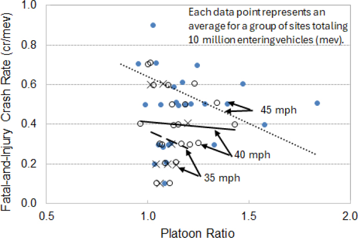
Platoon Ratio.
The association between platoon ratio and FI crash rate is shown in Figure 15. The trend lines shown represent a best-fit to the data points based on linear regression. The data are grouped into three speed limit categories to allow for a more focused examination of platoon ratio and crash rate. The trend suggests that, within each speed limit category, FI crash rate ratio is lower for those intersection legs with a larger platoon ratio (i.e., more favorable progression). This trend is consistent with that noted by Kabir et al. (2021). They examined crash frequency and percent-arrivals-on-green for 121 signalized intersections in Ohio. They found that a one percent increase in the percent-arrivals-on-green is associated with a 1.12 percent reduction in total crash frequency.
Entry During Red.
The association between the proportion-of-approach-volume-entering-during-the-through-red-interval (PVR) and crash rate is shown in Figure 16. The trend line shown is a line of best-fit to the data points based on linear regression. The trend shown suggests that crash rate is smaller for those sites with a larger PVR. This trend is contrary to results reported by Bonneson et al. (2002). Specifically, they compared the violation rate observed during one six-hour day at 12 intersection approaches with the three-year crash history for these approaches. They found that the frequency of right-angle and left-turn-opposed crashes was higher on those approaches with higher red-light violation rates.
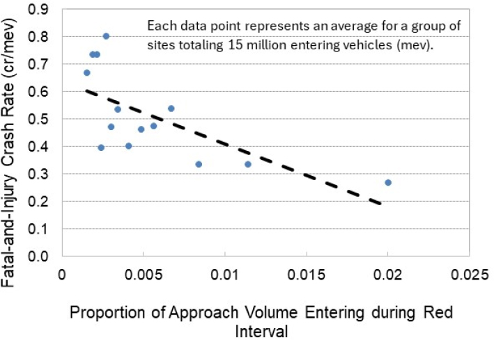
The trend shown in Figure 16 may reflect an unknown number of right-turn-on-red maneuvers that were counted by the ATSPM system (discussions with the UDOT staff also highlighted potential issues with the red actuation metric due to the detection issues related to both latency and the speed restriction feature that is typically used to eliminate right-turn-on-red maneuvers). These maneuvers are frequent in number and tend to be associated with fewer crashes than are vehicles that cross straight through the intersection during the red interval. Further investigation revealed that PVR is larger during periods with a lower traffic volume, which corresponds to larger gaps for the right-turn driver and less crash risk.
Entry During Yellow.
The association between the proportion-of-approach-volume-entering-during-the-through-yellow-interval (PVY) and crash rate is shown in Figure 17. The trend line shown is a line of best-fit to the data points based on linear regression. The trend shown suggests that crash rate is higher for those sites with a larger PVY. This trend is consistent with the findings of Yuan et al. (2020) who studied 42 signalized intersection approaches in Florida. They found that the odds of crash occurrence are higher when the arrival flow rate during the yellow indication is higher.
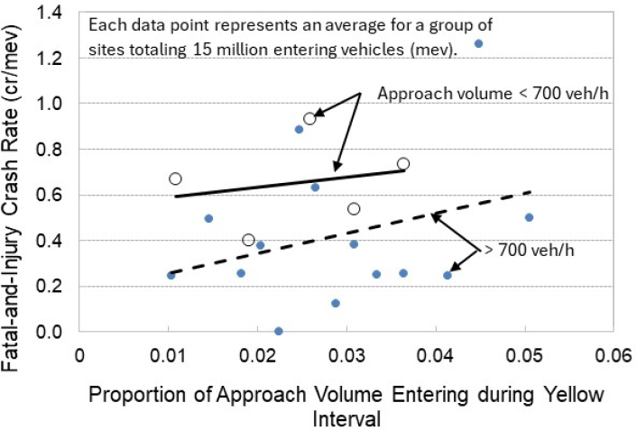
The two trend lines in Figure 17 indicate that the crash rate is higher for legs with lower volume. This trend may reflect the fact that high-volume legs are more likely to have favorable progression. As indicated in Figure 15, legs with favorable progression have a lower crash rate.
Split Failure.
The association between the proportion-of-cycles-with-through-phase-split-failure (PCFth) and crash rate is shown in Figure 18a. The trend line shown suggests that crash rate is slightly higher for those sites with a larger PCFth.
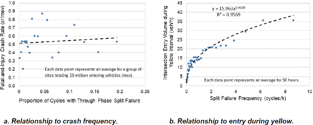
The trend line in Figure 18b shows the relationship between split failure frequency (SFF) and intersection-entry-volume-during-the-yellow-interval (EVY). The value of SFF is computed for each site by multiplying its PCF by the number of signal cycles per hour. The value of EVY is computed by multiplying PVY by the hourly volume. These computed values fairly compare the two measures on the basis of “events per hour”. They indicate that EVY and SFF are strongly correlated such that it may not be possible to include both variables (in separate AFs) in a multiple-AF model framework (i.e., Equation 21).
Permissive Left-Turn Measures.
The association between the proportion-of-through-green-interval-with-long-gaps (PGG) and crash rate is shown in Figure 19a. The trend line shown is a line of best-fit to the data points based on linear regression. The trend line shown indicates that crash rate is slightly higher for those sites with a small PGG.

The association between the left-turn permissive capacity and crash rate is shown in Figure 19b. The trend line shown indicates that crash rate is higher for those sites with a small left-turn permissive capacity.
When comparing the trends in Figure 19a and Figure 19b, it appears that the trend in Figure 19b provides a better fit to the data. This finding suggests that an AF based on permissive capacity may provide more reliable predictions than an AF based on PGG.
Case B CMF ‒ Cross-Sectional Study Statistical Analysis Methods
This section summarizes the statistical analysis methods used to estimate the regression model coefficients and the associated SPFs and AFs. The following topics are addressed in this section:
- Modeling Approach
- Statistical Analysis Methods
- Analysis of Percent-Arrivals-on-Green, Split Failures, and Yellow Actuations
- Analysis of Left-Turn Gaps
Modeling Approach
Two Models.
The composition of the database assembled for model estimation dictated the model framework that was used to estimate the CPMs and associated ATSPM-related AFs. Notably, a review of the study-site counts shown in Table 42 indicated that the data were capable of supporting the development of a multiple-AF model framework for three ATSPM reports (i.e., percent-arrivals-on-green, split failure frequency, and yellow-and-red actuations). In contrast, the data would support only a one-AF model framework for left-turn gap availability report. In summary, the following two models were developed:
- Multiple-AF model including SPF and AFs reflecting percent-arrivals-on-green, split failure frequency, and yellow-and-red actuations.
- One-AF model including SPF and AF reflecting left-turn gap availability.
The SPFs and AFs for both models were estimated using regression analysis of the data assembled for 109 sites in three states. The basic unit of analysis (i.e., the “observation”) is one hour of the typical weekday over the duration of one year at one site. The number of observations associated with each model are indicated at the bottom of Table 46 and Table 47. Thus, the models are developed to predict the annual average crash frequency for a specified hour of a typical weekday at one site.
Method of Accounting for Left-Turn and Through Phase Split Failures.
The database included data describing the proportion-of-cycles-with-split-failure for the phase serving the through (and right-turn) movement and for the phase serving the left-turn movement. Alternative model forms were investigated to determine how these two ATSPM reports could be used to provide the most reliable AF estimates. Based on a series of preliminary regression analyses, it was determined that an AF having a variable representing the probability-of-a-vehicle-experiencing-a-split-failure-on-the-subject-leg provided the best fit to the data. This variable was computed using the following equation.
| Equation 25 |
where,
| psf = | probability of a vehicle experiencing a split failure on the subject leg; |
| Pth = | proportion of approach volume traveling through or turning right; |
| Plt = | proportion of approach volume turning left or making a U-turn (= 1 – Pth); |
| PCFth = | proportion of cycles with through phase split failure; and |
| PCFlt = | proportion of cycles with left-turn phase split failure. |
The turn movement proportions needed for Equation 25 were not available in the database, so default values of Plt = 0.1 and Pth = 0.9 were used for all sites.
Red Actuations.
A preliminary regression analysis was undertaken to test the findings from the exploratory analysis related to red actuations. Based on this analysis, it was confirmed that red actuations are related to crash frequency in the illogical manner shown in Figure 16. It was rationalized that this trend may be skewed by frequent (and relatively safe) right-turn-on-red maneuvers represented in the red-actuations variable. For these reasons, the proportion-of-approach-volume-entering-during-the-through-red-interval (PVR) variable was not included in the model and an AF was not developed for it.
Hybrid Variables.
The preliminary regression analysis confirmed that platoon-ratio and left-turn-permissive-capacity were more reliable predictors of crash frequency, so they were the focus of AF development. As a result, the variables for proportion-of-approach-volume-arriving-during-the-through-green-interval (PVG) and proportion-of-through-green-interval-with-long-gaps (PGG) were not directly included in the AFs (rather, they were indirectly included via platoon ratio and left-turn capacity).
Approach for Addressing Correlation Between Yellow Actuations and Split Failure.
The preliminary regression analysis also confirmed that split failure frequency was highly correlated with entry volume during the yellow interval, as noted in the discussion of Figure 18b. For this reason, the multiple-AF model could not include both variables (and associated AFs). As a result, the researchers developed a multiple-AF model that included an AF for platoon ratio and an AF for the probability-of-a-vehicle-experiencing-a-split-failure (psf). The SPF and AF for platoon ratio where then used in a second regression analysis to estimate an AF for the proportion-of-approach-volume-entering-the-intersection-during-the-through-yellow-interval (PVY). In this manner, a multiple-AF model is available to the analyst to evaluate the combined safety effect of psf and platoon ratio, and a second multiple-AF model is available to the analyst to evaluate the combined safety effect of PVY and platoon ratio. Both models use the same SPF and platoon ratio AF.
Variables Considered but Not Included in Model.
A preliminary regression analysis was undertaken to test the findings from the exploratory data analysis and to determine if other variables in the database were associated with crash frequency. The results indicated that number-of-lanes and median-type did not have a logical or statistically significant association with crash risk in the assembled data. As a result, these variables are not included in the models. These findings are based on the site sample sizes used for model estimation, it is possible that a larger site sample could reveal that one or more of these factors does have a logical and statistically valid association with crash frequency.
Statistical Analysis Methods
The nonlinear regression procedure (NLMIXED) in the SAS System was used to estimate the proposed model coefficients. This procedure was used because variations of the proposed predictive model were nonlinear and unsuitable for the log-linear form used by many procedures that support regression analysis of non-negative count data. Specifically, the proposed model form has constructs that are not amenable to a log-linear structure.
Similar to the approach taken by Bonneson et al., (2021), the log-likelihood function for the negative multinomial distribution was used in NLMIXED to determine the best-fit model coefficients. As noted by Hauer (2004), the negative multinomial distribution is appropriate when (a) the negative binomial distribution adequately describes the crash distribution among a group of similar sites and (b) the measured site characteristics (e.g., traffic volume, signal timing, cycle length, etc.) change over time. The procedure was set up to estimate model coefficients based on maximum-likelihood methods, which was also described in Bonneson et al., (2008).
Use of the negative multinomial distribution in the analysis of the assembled database allows the regression model to be fit to each “annual hour” observation at each site while accounting for the correlated nature of the measured site characteristics among successive time periods. In statistical parlance, these observations are considered “repeated measures.” By accounting for these “repeated measures” in the
regression analysis, the resulting standard error estimates are more precise, and the associated statistical tests are more efficient.
Overdispersion Parameter
It was assumed that site crash frequency is Poisson distributed, and that the distribution of the mean crash frequency for a group of similar sites is gamma distributed. In this manner, the distribution of crashes for a group of similar sites can be described by the negative binomial distribution (also known as a Poisson-Gamma mixture distribution). The variance of this distribution is computed using the following equation.
| Equation 26 |
where,
| V[X] = | crash frequency variance for a group of similar sites (crashes2); |
| Np = | predicted average crash frequency (crashes/yr); |
| X = | reported crash count (crashes); and |
| φ = | inverse dispersion parameter. |
The overdispersion parameter k, as defined and used in the HSM, is computed using the following equation:
| Equation 27 |
where k = overdispersion parameter and φ = inverse dispersion parameter.
Model Fit Statistics
Three statistics were used to assess CPM fit to the data. One measure of fit is the Pearson χ2 statistic. This statistic is calculated using the following equation.
| Equation 28 |
where,
| χ2 = | Pearson chi-square statistic; |
| n = | number of observations; |
| V[Xi] = | crash frequency variance for a group of similar sites (crashes2); |
| Np,i = | predicted average crash frequency for observation i (crashes/h); and |
| Xi = | reported crash count for observation i (crashes). |
This statistic follows the χ2 distribution with n – p degrees of freedom, where n is the number of observations and p is the number of model variables (McCullagh and Nelder, 1983). This statistic is asymptotic to the χ2 distribution for larger sample sizes.
The second measure of model fit is the scale parameter φ. It is used to assess the amount of variation in the observed data, relative to the specified distribution. This statistic is calculated by dividing Equation 18 by the quantity n – p. A scale parameter near 1.0 indicates that the assumed distribution of the dependent variable is approximately equivalent to that found in the data. In this instance, a value near 1.0 indicates that negative binomial distribution adequately describes the crash distribution among the study sites.
The third measure of model fit is the pseudo R2 developed by McFadden (1974). This statistic provides a useful measure of model fit for maximum-likelihood regression. The pseudo R2 compares the log likelihood value for the estimated model with that for the “null” model. The null model includes only an intercept term (i.e., no predictor variables). The pseudo R2 is computed using the following equation.
| Equation 29 |
where
| Rp2 = | pseudo R2; |
| LLmodel = | log-likelihood for the estimated model; and |
| LLnull = | log-likelihood for the null model. |
Pseudo R2 values can range from 0.0 to 1.0, with larger values indicating a better fit to the data. This interpretation is similar to that for the traditional R2 metric based on ordinary least squares. However, unlike the traditional R2, typical values for the pseudo R2 range from 0.0 to 0.4, with values in the range of 0.2 to 0.4 indicating a very good fit (McFadden, 1977).
Analysis of Percent-Arrivals-on-Green, Split Failures, and Yellow Actuations
This section describes a set of CPMs that relate three ATSPM reports to crash frequency. It also presents the results from the model estimation process.
Model Development
Two CPMs were developed to describe the safety effect of percent-arrivals-on-green, split failures, and yellow actuations. One CPM predicts the frequency of fatal-and-injury (FI) crashes. The other CPM predicts the frequency of property-damage-only (PDO) crashes.
The functional form of (and independent variables in) the CPM for predicting FI crash frequency is the same as that for predicting PDO crash frequency. However, the model’s regression coefficients vary depending on whether the model is applied to FI or PDO crashes.
As noted in a previous section, split failure frequency is strongly correlated with yellow actuations such that both variables cannot be included in the same regression model. To overcome this issue, two regression analyses were undertaken. In the first analysis, the researchers estimated the coefficients for a model that included an AF for platoon ratio and an AF for the probability-of-a-vehicle-experiencing-a-split-failure psf. In the second analysis, the SPF and AF for platoon ratio where then used in a second regression analysis to estimate an AF for the proportion-of-approach-volume-entering-the-intersection-during-the-through-yellow-interval (PVY). These two models are described in the following paragraphs.
Regression Analysis 1.
The form of the regression model that included platoon ratio and split failure terms is described by the following equations.
| Equation 30 |
with
| Equation 31 |
| Equation 32 |
| Equation 33 |
| Equation 34 |
| Equation 35 |
| Equation 36 |
where,
| Np,i = | predicted average crash frequency during hour i of the typical day for the subject intersection leg (i = 0 to 23) (crashes/yr); |
| Nspf,i = | predicted average crash frequency for base conditions during hour i of the typical day for the subject intersection leg (i = 0 to 23) (crashes/yr); |
| AFRp,i = | adjustment factor for platoon ratio for hour i; |
| AFpk,i = | adjustment factor for peak traffic hour i; |
| AFsf,i = | adjustment factor for split failure for hour i; |
| AAHTa,i = | annual average hourly traffic volume for the approach lanes during hour i (veh/h); |
| It,j = | indicator variable for year of data (j = 2021, 2022, or 2023) (= 1 if data is for year j; 0 otherwise); |
| Ipk,j = | indicator variable for hour i as a peak traffic hour (= 1 if hour is in the range 7:00 to 9:00 am or 4:00 to 6:00 pm, 0 otherwise); |
| Rp,i = | platoon ratio for hour i; |
| Ci = | cycle length relative to the end of the through green interval during hour i; |
| Pi = | proportion of approach volume arriving during the through green interval during hour i; |
| (g/C)i = | proportion of cycle during the through green interval during hour i; |
| psf,i = | probability of a vehicle experiencing a split failure on the subject leg during hour i; |
| Pth,i = | proportion of approach volume traveling through or turning right during hour i (= 0.9); |
| Plt,i = | proportion of approach volume turning left or making a U-turn during hour i (= 0.1); |
| PCFth,i = | proportion of cycles with through phase split failure during hour i; |
| PCFlt,i = | proportion of cycles with left-turn phase split failure during hour i; and |
| bxyz = | regression coefficient, where the subscript is used to denote a specific variable. |
The fraction “5/7” in Equation 30 is an offset variable that recognizes the dependent variable in the estimation data represents weekday crash counts (i.e., Monday through Friday).
All of the variables associated with Equation 30 describe the traffic and signal timing characteristics for a specified leg at a signalized intersection of interest. The underlined variables were obtained from the ATSPM reports for the study sites represented in the estimation database.
The base conditions for this model are identified in the following list:
- Platoon ratio: 1.0
- Proportion of cycles with through phase split failure: 0.0
- Proportion of cycles with left-turn phase split failure: 0.0
- Traffic period: off-peak hour (peak hours: 7:00 to 9:00 am and 4:00 to 6:00 pm)
By definition, an AF has a value of 1.0 when its input variable(s) are at base-condition value(s).
The final form of the regression model is described by the preceding equations. This form reflects the findings from several preliminary regression analyses where alternative model forms were examined. The form that is described herein represents that which provided the best fit to the data.
Regression Analysis 2.
The form of the regression model that included the yellow actuation term is described by the following equations.
| Equation 37 |
with
| Equation 38 |
where
| = | computed average intersection leg crash frequency for base conditions during hour i using Equation 31 with estimation coefficients from regression analysis 1 (crashes/yr); |
| = | computed adjustment factor for platoon ratio for hour i using Equation 32 with estimation coefficients from regression analysis 1; |
| = | computed adjustment factor for peak traffic hour i using Equation 33 with estimation coefficients from regression analysis 1; |
| AFya,i = | adjustment factor for yellow actuations for hour i; |
| PVYi = | proportion of approach volume entering the intersection during the through yellow interval during hour i; |
and all other variables are as previously defined.
All of the variables associated with Equation 37 describe the traffic and signal timing characteristics for a specified leg at a signalized intersection of interest. The underlined variable was obtained from the ATSPM yellow-and-red actuations report for the study sites represented in the estimation database.
The base conditions for this model are identified in the following list:
- Platoon ratio: 1.0
- Proportion of approach volume entering during the through yellow interval: 0.0
- Traffic period: off-peak hour (peak hours: 7:00 to 9:00 am and 4:00 to 6:00 pm)
The final form of the regression model is described by the preceding equations. This form reflects the findings from several preliminary regression analyses where alternative model forms were examined. The form that is described herein represents that which provided the best fit to the data.
Model Estimation
This section summarizes the results of the regression model estimation for both regression analysis 1 and 2, as described in the previous section.
Regression Analysis 1.
This subsection describes the results of the regression model estimation for the CPMs that include the split failure and platoon ratio AFs. A total of 23 sites had the platoon ratio and split failure data needed to estimate this model.
The results for the FI-crash model are presented in Table 50. The Pearson χ2 statistic for the model is 1695, and the degrees of freedom are 1603 (= n − p = 1608 − 5). Only one intercept variable is counted towards the value of p for this calculation given the intercept’s use in the negative multinomial error distribution. As this statistic is less than χ20.05, 1603 (= 1697), the hypothesis that the model fits the data cannot be rejected. The Rp2 for the model is 0.11. As described in a previous section, typical values for the pseudo R2 range from 0.0 to 0.4, with values in the range of 0.2 to 0.4 indicating a very good fit (McFadden, 1977).
Table 50. Predictive model estimation statistics ‒ FI crashes, platoon ratio and split failure.
| Model Statistics Value | ||||
|---|---|---|---|---|
| Scale Parameter φ: | 1.06 | |||
| Pearson χ2: | 1695 (χ20.05, 1603 = 1697) | |||
| Pseudo R2: | 0.11 | |||
| Observations n: | 1608 one-hour periods (98 FI crashes) | |||
| Estimated Coefficient Values | ||||
| Variable | Description | Value | Std. Error | t-statistic |
| b0,21 | Intercept for Year 2021 | -2.005 | 0.306 | -6.55 |
| b0,22 | Intercept for Year 2022 | -1.993 | 0.294 | -6.78 |
| b0,23 | Intercept for Year 2023 | -2.016 | 0.290 | -6.94 |
| bvol | Approach AAHT volume | 1.018 | 0.241 | 4.23 |
| bRp | Platoon ratio | -2.070 | 0.961 | -2.15 |
| bsf | Split failure | 0.397 | 0.223 | 1.78 |
| bpk | Peak hour indicator variable | -0.356 | 0.249 | -1.43 |
| k | Overdispersion parameter | 0.450 | 0.206 | 2.18 |
The t-statistics listed in the last column of Table 50 indicate a test of the null hypothesis that the coefficient value is equal to 0.0. Those t-statistics with an absolute value that is larger than 1.96 indicate that the hypothesis can be rejected with the probability of error in this conclusion being less than 0.05.
A second t-statistic threshold was established for those AF variables that were important to the model and whose AF trend was found to be logical and consistent with intuition or previous research findings. Coefficients associated with variables of this nature were tested against the t-statistic value of 1.4, which corresponds to a probability of error in rejecting the null hypothesis of 0.16. A coefficient where the absolute value of the t-statistic was between 1.4 and 1.96, that was important to the model, and whose trend was found to be logical and consistent with intuition or previous research findings was also retained in the CPM.
The fit of the estimated model is shown in Figure 20. The model was applied to each of the 23 sites (i.e., intersection legs) in the database. To create this figure, the predicted crash frequency was computed for each hour of the typical day at each site and the results added for all 24 hours. Each data point shown represents the average predicted and average reported FI crash frequency for a group of 3 sites. In general, the data shown in the figure indicate that the model provides an unbiased estimate of predicted crash frequency for sites experiencing up to 2.5 FI crashes/year.
The results for the PDO-crash model are presented in Table 51. The Pearson χ2 statistic for the model is 1582, and the degrees of freedom are 1604 (= n − p = 1608 − 4). As this statistic is less than χ20.05, 1604 (= 1698), the hypothesis that the model fits the data cannot be rejected. The Rp2 for the model is 0.13.
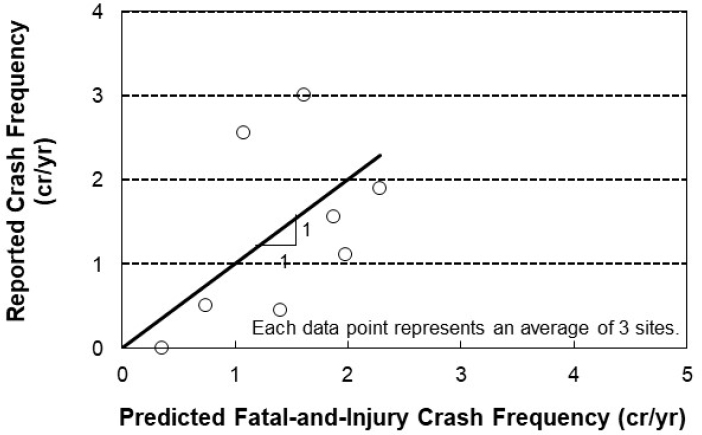
Table 51. Predictive model estimation statistics ‒ PDO crashes, platoon ratio and split failures.
| Model Statistics Value | ||||
|---|---|---|---|---|
| Scale Parameter φ: | 0.98 | |||
| Pearson χ2: | 1582 (χ20.05, 1604 = 1698) | |||
| Pseudo R2: | 0.13 | |||
| Observations n: | 1608 one-hour periods (237 PDO crashes) | |||
| Estimated Coefficient Values | ||||
| Variable | Description | Value | Std. Error | t-statistic |
| b0,21 | Intercept for Year 2021 | -1.198 | 0.213 | -5.63 |
| b0,22 | Intercept for Year 2022 | -1.447 | 0.213 | -6.78 |
| b0,23 | Intercept for Year 2023 | -1.307 | 0.206 | -6.34 |
| bvol | Approach AAHT volume | 0.965 | 0.146 | 6.62 |
| bRp | Platoon ratio | -0.815 | 0.522 | -1.56 |
| bsf | Split failure | 0.341 | 0.138 | 2.47 |
| bpk | Peak hour indicator variable | n.s. | n.s. | n.s. |
| k | Overdispersion parameter | 0.358 | 0.131 | 2.73 |
n.s. – coefficient is not statistically significant (and is excluded from the model).
The t-statistics listed in the last column of Table 51 indicate a test of the null hypothesis that the coefficient value is equal to 0.0. Those t-statistics with an absolute value that is larger than 1.96 indicate that the hypothesis can be rejected with the probability of error in this conclusion being less than 0.05. As noted previously, a coefficient where the absolute value of the t-statistic was between 1.4 and 1.96, that was important to the model, and whose trend was found to be logical and consistent with intuition or previous research findings was also retained in the CPM.
The coefficient for the peak hour indicator variable was not statistically significant. As a result, it was removed from the model. The CPM for predicting PDO crash frequency does not include the adjustment factor for peak traffic hour AFpk.
The fit of the estimated model is shown in Figure 21. The model was applied to each of the 23 sites (i.e., intersection legs) in the database. Each data point shown represents the average predicted and average reported PDO crash frequency for a group of 3 sites. In general, the data shown in the figure indicate that the model provides an unbiased estimate of predicted crash frequency for sites experiencing up to 6.0 PDO crashes/year.

Regression Analysis 2.
This subsection describes the results of the regression model estimation for the CPM that includes the yellow actuation AF. Two sites in North Carolina did not have the necessary yellow actuation data for this analysis, leaving 21 sites for model estimation.
The results for the FI-crash model are presented in Table 52. The Pearson χ2 statistic for the model is 1483, and the degrees of freedom are 1511 (= n − p = 1512 − 1). As this statistic is less than χ20.05, 1511 (= 1602), the hypothesis that the model fits the data cannot be rejected. The Rp2 for the model is 0.11.
Table 52. Predictive model estimation statistics ‒ FI crashes, yellow actuations.
| Model Statistics Value | ||||
|---|---|---|---|---|
| Scale Parameter φ: | 0.98 | |||
| Pearson χ2: | 1483 (χ20.05, 1511 = 1602) | |||
| Pseudo R2: | 0.11 | |||
| Observations n: | 1512 one-hour periods (95 FI crashes) | |||
| Estimated Coefficient Values | ||||
| Variable | Description | Value | Std. Error | t-statistic |
| bya | Yellow actuations | 0.285 | 0.100 | 2.85 |
| k | Overdispersion parameter | 0.519 | 0.230 | 2.26 |
The t-statistics listed in the last column of Table 52 indicate a test of the null hypothesis that the coefficient value is equal to 0.0. Those t-statistics with an absolute value that is larger than 1.96 indicate that the hypothesis can be rejected with the probability of error in this conclusion being less than 0.05.
The fit of the estimated model is shown in Figure 22. The model was applied to each of the 21 sites in the database. Each data point shown represents the average predicted and average reported FI crash frequency for a group of 3 sites. In general, the data shown in the figure indicate that the model provides an unbiased estimate of predicted crash frequency for sites experiencing up to 2.5 FI crashes/year.
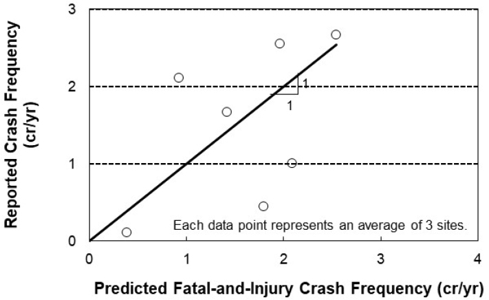
The results for the PDO-crash model are presented in Table 53. The Pearson χ2 statistic for the model is 1600, and the degrees of freedom are 1511 (= n − p = 1512 − 1). As this statistic is less than χ20.05, 1511 (= 1602), the hypothesis that the model fits the data cannot be rejected. The Rp2 for the model is 0.13.
Table 53. Predictive model estimation statistics ‒ PDO crashes, yellow actuations.
| Model Statistics Value | ||||
|---|---|---|---|---|
| Scale Parameter φ: | 1.06 | |||
| Pearson χ2: | 1600 (χ20.05, 1511 = 1602) | |||
| Pseudo R2: | 0.13 | |||
| Observations n: | 1512 one-hour periods (221 PDO crashes) | |||
| Estimated Coefficient Values | ||||
| Variable | Description | Value | Std. Error | t-statistic |
| bya | Yellow actuations | 0.253 | 0.078 | 3.23 |
| k | Overdispersion parameter | 0.427 | 0.156 | 2.73 |
The t-statistics listed in the last column of Table 53 indicate a test of the null hypothesis that the coefficient value is equal to 0.0. Those t-statistics with an absolute value that is larger than 1.96 indicate that the hypothesis can be rejected with the probability of error in this conclusion being less than 0.05.
The coefficient for the peak hour indicator variable was not statistically significant in the PDO model estimated in regression analysis 1. As a result, the CPM for predicting PDO crash frequency in regression analysis 2 does not include the adjustment factor for peak traffic hour AFpk.
The fit of the estimated model is shown in Figure 23. The model was applied to each of the 21 sites in the database. Each data point shown represents the average predicted and average reported PDO crash frequency for a group of 3 sites. In general, the data shown in the figure indicate that the model provides an unbiased estimate of predicted crash frequency for sites experiencing up to 6.0 PDO crashes/year.
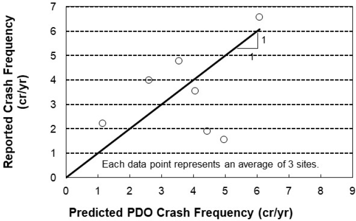
Analysis of Left-Turn Gaps
This section describes a CPM that relates left-turn-gap-availability to crash frequency. It also presents the results from the model estimation process. The models are applicable only intersection legs that have an opposing left-turn movement that is served by permissive or protected/permissive left-turn operation.
Model Development
Two CPMs were developed to describe the safety effect of left-turn gap availability. One CPM predicts the frequency of left-turn-with-opposing-through-vehicle (LT) crashes (all severities). The other CPM predicts the frequency of all other (nonLT) crashes (all severities). Both models are developed using 23 sites for which the left-turn movement opposing the subject leg is served by permissive or protected/permissive left-turn operation.
The model for predicting LT crash frequency is the primary product of this development. It is intended to be used by analysts when evaluating the safety effect of alternative signal timing strategies that change left-turn gap availability. In contrast, the model for predicting nonLT crash frequency was primarily developed to confirm whether changes to left-turn gap-availability have an adverse effect on intersection safety. As a matter of good practice, before an analyst implements a treatment to reduce target crashes, he or she should first confirm that the treatment will not inadvertently increase non-target crashes. The nonLT CPM was developed to support this practice.
The functional form of (and independent variables in) the CPM for predicting LT crash frequency is the same as that for predicting nonLT crash frequency. However, the model’s regression coefficients vary
depending on whether the model is applied to LT or nonLT crashes. These two models are described in the following equations.
| Equation 39 |
with
| Equation 40 |
| Equation 41 |
| Equation 42 |
where,
| Np,i = | predicted average crash frequency during hour i of the typical day for the subject intersection leg (i = 0 to 23) (crashes/yr); |
| Nspf,i = | predicted average crash frequency for base conditions during hour i of the typical day for the subject intersection leg (i = 0 to 23) (crashes/yr); |
| AFlt,i = | adjustment factor for left-turn permissive capacity for hour i; |
| AAHTa,i = | annual average hourly traffic volume for the approach lanes during hour i (veh/h); |
| It,j = | indicator variable for year of data (j = 2021, 2022, or 2023) (= 1 if data is for year j; 0 otherwise). |
| Sp = | approach speed limit (mph); |
| clt,perm,i = | opposing left-turn permissive capacity during hour i (veh/h); |
| Plt,g,i = | proportion of the through green interval with long gaps in the through traffic stream for hour i; |
| (g/C)i = | proportion of cycle during the through green interval during hour i; and |
| bxyz = | regression coefficient, where the subscript is used to denote a specific variable. |
The fraction “5/7” in Equation 39 is an offset variable that recognizes the dependent variable in the estimation data represents weekday crash counts (i.e., Monday through Friday).
All of the variables associated with Equation 39 describe the traffic and signal timing characteristics for a specified leg at a signalized intersection of interest. The underlined variables were obtained from the ATSPM reports for the study sites represented in the estimation database.
The model variables describe the leg of interest. Notably, the proportions Plt,g,i and (g/C)i describe the through traffic stream for the subject leg (not the opposing leg).
The base conditions for this model are identified in the following list:
- Approach speed limit: 40 mph
- Opposing left-turn permissive capacity: 1000 veh/h
The final form of the regression model is described by the preceding equations. This form reflects the findings from several preliminary regression analyses where alternative model forms were examined. The form that is described herein represents that which provided the best fit to the data.
Model Estimation
This section describes the results of the regression model estimation for the CPMs that include the left-turn gap availability AF. A total of 23 sites had the left-turn gap availability data needed to estimate this model. However, one site was identified as an outlier during a preliminary regression analysis. It was the
east leg of signal 7540, which was first noted in the discussion associated with Table 49. This site was removed from the data, leaving 22 sites in the estimation database.
The results for the LT-crash model are presented in Table 54. The Pearson χ2 statistic for the model is 1508, and the degrees of freedom are 1556 (= n − p = 1560 − 4). Only one intercept variable is counted towards the value of p for this calculation given the intercept’s use in the negative multinomial error distribution. As this statistic is less than χ20.05, 1556 (= 1649), the hypothesis that the model fits the data cannot be rejected. The Rp2 for the model is 0.09. As described in a previous section, typical values for the pseudo R2 range from 0.0 to 0.4, with values in the range of 0.2 to 0.4 indicating a very good fit (McFadden, 1977).
Table 54. Predictive model estimation statistics ‒ Left-turn-opposed crashes, gap availability.
| Model Statistics Value | ||||
|---|---|---|---|---|
| Scale Parameter φ: | 0.97 | |||
| Pearson χ2: | 1508 (χ20.05, 1556 = 1649) | |||
| Pseudo R2: | 0.09 | |||
| Observations n: | 1560 one-hour periods (62 LT crashes) | |||
| Estimated Coefficient Values | ||||
| Variable | Description | Value | Std. Error | t-statistic |
| b0,21 | Intercept for Year 2021 | -3.273 | 0.522 | -6.27 |
| b0,22 | Intercept for Year 2022 | -3.126 | 0.546 | -5.72 |
| b0,23 | Intercept for Year 2023 | -3.298 | 0.552 | -5.97 |
| bvol | Approach AAHT volume | 0.873 | 0.323 | 2.70 |
| bcap | Left-turn capacity | -0.637 | 0.406 | -1.57 |
| bsp | Speed limit | -0.0885 | 0.0525 | -1.69 |
| k | Overdispersion parameter | 0.554 | 0.343 | 1.62 |
The t-statistics listed in the last column of Table 54 indicate a test of the null hypothesis that the coefficient value is equal to 0.0. Those t-statistics with an absolute value that is larger than 1.96 indicate that the hypothesis can be rejected with the probability of error in this conclusion being less than 0.05.
A second t-statistic threshold was established for those AF variables that were important to the model and whose AF trend was found to be logical and consistent with intuition or previous research findings. Coefficients associated with variables of this nature were tested against the t-statistic value of 1.4, which corresponds to a probability of error in rejecting the null hypothesis of 0.16. A coefficient where the absolute value of the t-statistic was between 1.4 and 1.96, that was important to the model, and whose trend was found to be logical and consistent with intuition or previous research findings was also retained in the CPM.
The left-turn capacity coefficient in Table 54, when used Equation 41, indicates that crash risk is higher at sites with a lower left-turn capacity. The speed limit coefficient indicates that the change in crash risk with a change in capacity is higher for sites with a higher speed limit.
The fit of the estimated model is shown in Figure 24. The model was applied to each of the 22 sites (i.e., intersection legs) in the database. To create this figure, the predicted crash frequency was computed for each hour of the typical day at each site and the results added for all 24 hours. Each data point shown represents the average predicted and average reported LT crash frequency for a group of 3 sites. In general, the data shown in the figure indicate that the model provides an unbiased estimate of predicted crash frequency for sites experiencing up to 1.7 LT crashes/year.
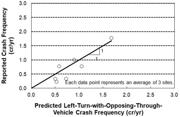
The results for the nonLT-crash model are presented in Table 55. The Pearson χ2 statistic for the model is 1640, and the degrees of freedom are 1556 (= n − p = 1560 − 4). As this statistic is less than χ20.05, 1556 (= 1649), the hypothesis that the model fits the data cannot be rejected. The Rp2 for the model is 0.13.
Table 55. Predictive model estimation statistics ‒ Non-left-turn opposed crashes, gap availability.
| Model Statistics Value | ||||
|---|---|---|---|---|
| Scale Parameter φ: | 1.05 | |||
| Pearson χ2: | 1,640 (χ20.05, 1556 = 1,649) | |||
| Pseudo R2: | 0.13 | |||
| Observations n: | 1,560 one-hour periods (376 nonLT crashes) | |||
| Estimated Coefficient Values | ||||
| Variable | Description | Value | Std. Error | t-statistic |
| b0,21 | Intercept for Year 2021 | -0.962 | 0.266 | -3.62 |
| b0,22 | Intercept for Year 2022 | -0.789 | 0.271 | -2.92 |
| b0,23 | Intercept for Year 2023 | -1.075 | 0.277 | -3.88 |
| bvol | Approach AAHT volume | 1.077 | 0.149 | 7.22 |
| bcap | Left-turn capacity | -0.309 | 0.189 | -1.63 |
| bsp | Speed limit | n.s. | n.s. | n.s. |
| k | Overdispersion parameter | 0.409 | 0.143 | 2.86 |
n.s. – coefficient is not statistically significant (and is excluded from the model).
The t-statistics listed in the last column of Table 55 indicate a test of the null hypothesis that the coefficient value is equal to 0.0. Those t-statistics with an absolute value that is larger than 1.96 indicate that the hypothesis can be rejected with the probability of error in this conclusion being less than 0.05. As noted previously, a coefficient where the absolute value of the t-statistic was between 1.4 and 1.96, that
was important to the model, and whose trend was found to be logical and consistent with intuition or previous research findings was also retained in the CPM.
The coefficient for the speed limit variable was not statistically significant. As a result, it was removed from the model. The AF for left-turn permissive capacity does not include this variable.
The fit of the estimated model is shown in Figure 25. The model was applied to each of the 22 sites (i.e., intersection legs) in the database. Each data point shown represents the average predicted and average reported nonLT crash frequency for a group of 3 sites. The trend in the data suggests that an unexplained systematic effect may remain in the data. A subsequent investigation did not reveal the source of the observed systematic trend. Nevertheless, the primary purpose of this CPM is to confirm that the correlation between capacity and LT crash frequency is the same as that for nonLT crash frequency (i.e., that an analyst that increases left-turn permissive capacity to reduce LT crash frequency does not inadvertently increase nonLT crash frequency). The negative value for the left-turn capacity coefficient bcap in Table 55 provides this confirmation.
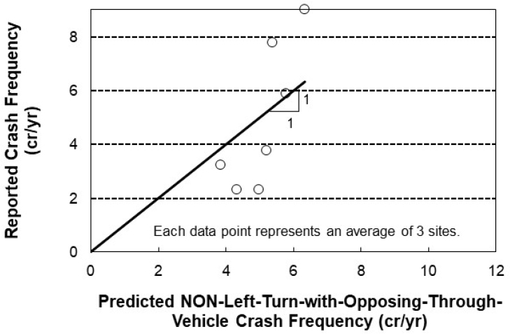
Case B CMF – Findings from Cross-Sectional Study
This section presents the estimated SPFs and AFs that comprise the set of CPMs developed for the project. The presentation of each CPM component includes the parametrized equations and a figure illustrating the sensitivity of the prediction to various independent variables.
Analysis of Percent-Arrivals-on-Green, Split Failures, and Yellow Actuations
This section presents the estimated CPMs for predicting the safety effect of percent-arrivals-on-green (as embodied in the platoon ratio variable), peak hour traffic conditions, split failure, and yellow actuations. One subsection describes the CPM for predicting FI crash frequency. The second subsection describes the CPM for predicting PDO crash frequency. The SPF and AF components of each CPM are described in the associated subsection.
- CPM for FI Crash Frequency
- CPM for PDO Crash Frequency
CPM for FI Crash Frequency
This section describes the CPM for predicting FI crash frequency. For each SPF and AF component of the CPM, the description includes one subsection that (a) presents the parameterized equation and (b) includes a figure illustrating equation trends. The CPM (and its SPF and AF components) is described by the following equation.
| Equation 43 |
where,
| Np,FI,i = | predicted average FI crash frequency during hour i of the typical day for the subject intersection leg (i = 0 to 23) (crashes/yr); |
| Nspf,FI,i = | predicted average FI crash frequency for base conditions during hour i of the typical day for the subject intersection leg (i = 0 to 23) (crashes/yr); |
| AFRp,FI,i = | FI SPF adjustment factor for platoon ratio for hour i; |
| AFpk,FI,i = | FI SPF adjustment factor for peak traffic hour i (peak hours: 7:00 to 9:00 am and 4:00 to 6:00 pm); |
| AFsf,FI,i = | FI SPF adjustment factor for split failure for hour i; |
| AFya,FI,i = | FI SPF adjustment factor for yellow actuations for hour i; and |
| Cf,FI = | FI SPF calibration factor. |
This equation is used to evaluate one specified hour for a given signalized intersection leg. The predicted value from the equation represents the annual average FI crash frequency for the specified hour. Multiple hours of the typical day can be evaluated by repeated application of the equation. The predicted average FI crash frequency for each hour can be added to estimate the average crash frequency for the combined set of hours.
There are two AFs listed in the parentheses of Equation 43. Only one of these two AF can be used when the CPM is applied to a site. This restriction reflects the fact that the two AF are highly correlated and tend to predict the risk associated with the same crash events.
If the operating conditions being evaluated exist only for a specific subset of the days of the typical week, then the predicted average crash frequency is multiplied by the number of applicable days per week and then divided by 7. For example, if the signal timing plan being evaluated applies only to weekdays (i.e., Monday to Friday), then the analyst would multiply the predicted average crash frequency by 5/7 (= 5 days per weekday/7 days per week).
Safety Performance Function.
The predicted average crash frequency for base conditions is described by the following equation.
| Equation 44 |
Where the AAHTa,i volume variable represents the annual average hourly volume during a specified hour i for the subject intersection leg. The coefficient “-2.016” corresponds to the Year 2023. The calibration factor Cf (to be provided by the analyst) will provide the necessary adjustments to ensure that the model predictions reflect the desired year of application and local conditions.
The SPF relationship between predicted FI crash frequency and hourly traffic volume is illustrated in Figure 26a. It is applicable to annual average hourly volumes as large as 1,200 veh/h but may be used with caution to evaluate volumes slightly larger than this value. The trend line indicates that intersection legs with higher volume have more frequent crashes.
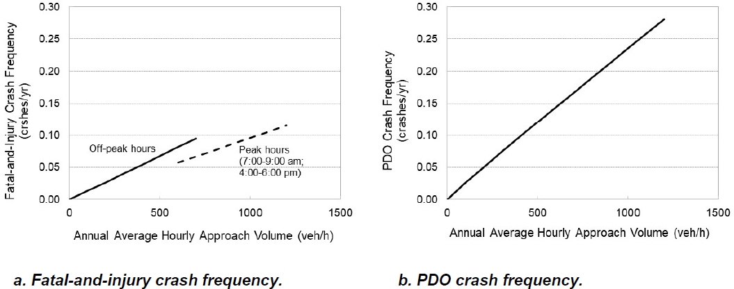
The solid trend line in Figure 26a illustrates the values obtained from Equation 44. The dashed trend line illustrates the values obtained from Equation 44 multiplied by the adjustment factor for the peak traffic hour AFpk. This adjustment factor is described in a subsequent paragraph.
The SPF relationship between predicted PDO crash frequency and hourly traffic volume is illustrated in Figure 26b. It is shown here to facilitate a comparison between the predicted FI and PDO crash frequencies. The SPF for predicting PDO crash frequency is described in the next section.
Adjustment Factor for Platoon Ratio.
The AF for platoon ratio is described by the following equation.
| Equation 45 |
Where Rp is the platoon ratio for hour i. The base condition for this adjustment factor is a platoon ratio of 1.0. It is applicable to platoon ratios in the range of 0.8 to 1.6.
The estimated AF trend for FI crash frequency is shown in Figure 27a. The trend line in this figure illustrates the values obtained from Equation 45. The trend indicates that intersection approaches with favorable progression have a lower crash risk than those approaches with unfavorable progression.
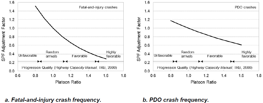
The estimated AF trend for PDO crash frequency is shown in Figure 27b. It is shown here to facilitate a comparison of the AF values for FI and PDO crashes. The AF for PDO crash frequency is described in the next section.
Adjustment Factor for Peak Traffic Hour.
The AF for peak traffic hour is described by the following equation.
| Equation 46 |
Where the indicator variable for hour i Ipk,j has a value of 1 if the subject hour is in the range 7:00 to 9:00 am or 4:00 to 6:00 pm. If it is not in this range, then the indicator variable value is 0. The value of this AF is 0.70 for peak traffic hours and 1.0 for off-peak hours.
Adjustment Factor for Split Failure.
The AF for split failure is described by the following equation.
| Equation 47 |
where,
| Ci = | cycle length relative to the end of the through green interval during hour i; and |
| psf,i = | probability of a vehicle experiencing a split failure on the subject leg during hour i. |
The probability of a vehicle experiencing a split failure psf,i is computed using Equation 36 (it is described in the discussion associated with Equation 25). The base condition for this AF is no split failures for the left-turn phase or the through phase serving the subject approach lanes. It is applicable to approaches where the probability of vehicle experiencing split failure ranges from 0.0 to 0.30.
The estimated AF trend for FI crash frequency is shown in Figure 28a. The trend line in this figure illustrates the values obtained from Equation 47. The trend indicates that intersection approaches with a higher probability of split failure have a higher crash risk. The trend shown in Figure 28b is discussed in the next section. For a given probability of split failure, the trends indicate that crash risk is lower for those legs with a larger cycle length.

Adjustment Factor for Yellow Actuations.
The AF for yellow actuations is described by the following equation.
| Equation 48 |
where,
| AAHTa,i = | annual average hourly traffic volume for the approach lanes during hour i (veh/h); and |
| PVYi = | proportion of approach volume entering the intersection during the through yellow interval during hour i. |
The base condition for this AF is no vehicles entering during the through yellow interval (i.e., PVYi = 0). It is applicable to approaches where the value of PVYi is less than 0.1.
The estimated AF trend for FI crash frequency is shown in Figure 29a. The trend line in this figure illustrates the values obtained from Equation 48. The trend indicates that, for a given approach volume, intersection approaches with a higher probability of intersection entry during yellow have a higher crash risk. For a given probability of entry, crash risk is shown to be higher for those approaches with higher volume. The trend shown in Figure 29b is discussed in the next section.
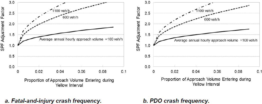
CPM for PDO Crash Frequency
This section describes the CPM for predicting PDO crash frequency. For each SPF and AF component of the CPM, the description includes one subsection that (a) presents the parameterized equation and (b) includes a figure illustrating equation trends. The CPM (and its SPF and AF components) is described by the following equation.
| Equation 49 |
where,
| Np,PDO,i = | predicted average PDO crash frequency during hour i of the typical day for the subject intersection leg (i = 0 to 23) (crashes/yr); |
| Nspf,PDO,i = | predicted average PDO crash frequency for base conditions during hour i of the typical day for the subject intersection leg (i = 0 to 23) (crashes/yr); |
| AFRp,PDO,i = | PDO SPF adjustment factor for platoon ratio for hour i; |
| AFsf,PDO,i = | PDO SPF adjustment factor for split failure for hour i; |
| AFya,PDO,i = | adjustment factor for yellow actuations for hour i; and |
| Cf,PDO = | PDO SPF calibration factor. |
This equation is used to evaluate one specified hour for a given signalized intersection leg. The predicted value represents the annual average PDO crash frequency for the specified hour. Multiple hours of the typical day can be evaluated by repeated application of the equation. The predicted average PDO crash frequency for each hour can be added to estimate the average crash frequency for the combined set of hours.
There are two AFs listed in the parentheses of Equation 49. Only one of these two AF can be used when the CPM is applied to a site. This restriction reflects the fact that the two AF are highly correlated and tend to predict the risk associated with the same crash events.
If the operating conditions being evaluated exist only for a specific subset of the days of the typical week, then the predicted average crash frequency is multiplied by the number of applicable days per week and then divided by 7. For example, if the signal timing plan being evaluated applies only to weekdays (i.e., Monday to Friday), then the analyst would multiply the predicted average crash frequency by 5/7 (= 5 days per weekday/7 days per week).
Safety Performance Function.
The predicted average crash frequency for base conditions is described by the following equation.
| Equation 50 |
Where the AAHTa,i volume variable represents the annual average hourly volume during a specified hour i for the subject intersection leg. The coefficient “-1.307” corresponds to the Year 2023. The calibration factor Cf (to be provided by the analyst) will provide the necessary adjustments to ensure that the model predictions reflect the desired year of application and local conditions.
The SPF relationship between predicted PDO crash frequency and hourly traffic volume is illustrated in Figure 26b. It is applicable to annual average hourly volumes as large as 1,200 veh/h but may be used with caution to evaluate volumes slightly larger than this value. The trend line indicates that intersection legs with higher volume have more frequent crashes.
Adjustment Factor for Platoon Ratio.
The AF for platoon ratio is described by the following equation.
| Equation 51 |
Where Rp is the platoon ratio for hour i. The base condition for this adjustment factor is a platoon ratio of 1.0. It is applicable to platoon ratios in the range of 0.8 to 1.6.
The estimated AF trend for PDO crash frequency is shown in Figure 27b. The trend line in this figure illustrates the values obtained from Equation 51. The trend indicates that intersection approaches with favorable progression have a lower crash risk than those approaches with unfavorable progression.
Adjustment Factor for Split Failure.
The AF for split failure is described by the following equation.
| Equation 52 |
where,
| Ci = | cycle length relative to the end of the through green interval during hour i; and |
| psf,i = | probability of a vehicle experiencing a split failure on the subject leg during hour i. |
The probability of a vehicle experiencing a split failure psf,i is computed using Equation 36. The base condition for this AF is no split failures for the left-turn phase or the through phase serving the subject approach lanes. It is applicable to approaches where the probability of vehicle experiencing split failure ranges from 0.0 to 0.30.
The estimated AF trend for PDO crash frequency is shown in Figure 28b. The trend line in this figure illustrates the values obtained from Equation 52. The trend indicates that intersection approaches with a higher probability of split failure have a higher crash risk. For a given probability of split failure, the trends indicate that crash risk is lower for those legs with a larger cycle length.
Adjustment Factor for Yellow Actuations.
The AF for yellow actuations is described by the following equation.
| Equation 53 |
where,
| AAHTa,i = | annual average hourly traffic volume for the approach lanes during hour i (veh/h); and |
| PVYi = | proportion of approach volume entering the intersection during the through yellow interval during hour i. |
The base condition for this AF is no vehicles entering during the through yellow interval (i.e., PVYi = 0). It is applicable to approaches where the value of PVYi is less than 0.1.
The estimated AF trend for PDO crash frequency is shown in Figure 29b. The trend line in this figure illustrates the values obtained from Equation 53. The trend indicates that, for a given approach volume, intersection approaches with a higher probability of intersection entry during yellow have a higher crash risk. For a given probability of entry, crash risk is shown to be higher for those approaches with higher volume.
Analysis of Left-Turn Gaps
This section presents the estimated CPMs for predicting the safety effect of left-turn gap availability. One subsection describes the CPM for predicting the frequency of left-turn-with-opposing-through-vehicle (LT) crashes. The second subsection describes the CPM for predicting the frequency of all other (nonLT) crashes. The SPF and AF components of each CPM are described in the associated subsection.
- CPM for Left-Turn-Opposed Crash Frequency
- CPM for NON-Left-Turn-Opposed Crash Frequency
CPM for Left-Turn-Opposed Crash Frequency
This section describes the CPM for predicting LT crash frequency (all severities). For each SPF and AF component of the CPM, the description includes one subsection that (a) presents the parameterized equation and (b) includes a figure illustrating equation trends. The CPM (and its SPF and AF components) is described by the following equation.
| Equation 54 |
where,
| Np,LT,i = | predicted average LT crash frequency during hour i of the typical day for the subject intersection leg (i = 0 to 23) (crashes/yr); |
| Nspf,LT,i = | predicted average LT crash frequency for base conditions during hour i of the typical day for the subject intersection leg (i = 0 to 23) (crashes/yr); |
| AFlt,LT,i = | LT SPF adjustment factor for left-turn permissive capacity for hour i; and |
| Cf,LT = | LT SPF calibration factor. |
This equation is used to evaluate one specified hour for a given signalized intersection leg. The intersection leg of interest must have an opposing left-turn movement that is served by permissive or protected/permissive left-turn operation.
The predicted value from the equation represents the annual average LT crash frequency for the specified hour. Multiple hours of the typical day can be evaluated by repeated application of the equation. The predicted average LT crash frequency for each hour can be added to estimate the average crash frequency for the combined set of hours.
If the operating conditions being evaluated exist only for a specific subset of the days of the typical week, then the predicted average crash frequency is multiplied by the number of applicable days per week and then divided by 7. For example, if the signal timing plan being evaluated applies only to weekdays (i.e., Monday to Friday), then the analyst would multiply the predicted average crash frequency by 5/7 (= 5 days per weekday/7 days per week).
Safety Performance Function.
The predicted average crash frequency for base conditions is described by the following equation.
| Equation 55 |
Where the AAHTa volume variable represents the annual average hourly volume during a specified hour i for the subject intersection leg. The coefficient “-3.298” corresponds to the Year 2023. The calibration factor Cf (to be provided by the analyst) will provide the necessary adjustments to ensure that the model predictions reflect the desired year of application and local conditions.
The SPF relationship between predicted LT crash frequency and hourly traffic volume is illustrated in Figure 30a. It is applicable to annual average hourly volumes as large as 1,200 veh/h but may be used with caution to evaluate volumes slightly larger than this value. The trend line indicates that intersection legs with higher volume have more frequent crashes.
The SPF relationship between predicted nonLT crash frequency and hourly traffic volume is illustrated in Figure 30b. It is shown here to facilitate a comparison between the predicted LT and nonLT crash frequencies. The SPF for predicting nonLT crash frequency is described in the next section.

Adjustment Factor for Left-Turn Gap Availability.
The AF for left-turn gap availability is described by the following equation.
| Equation 56 |
where,
| Sp = | approach speed limit (mph); and |
| clt,perm,i = | opposing left-turn permissive capacity during hour i (veh/h). |
The opposing left-turn permissive capacity variable is computed using Equation 42. The base conditions for this AF correspond to a speed limit of 40 mph and an opposing left-turn capacity of 1,000 veh/h. The AF applies to speed limits in the range of 30 to 50 mph. However, if the speed limit is less than 35 mph then a value of “35” should be used in the equation. Similarly, if the speed limit is more than 45 mph, then a value of “45” should be used in the equation. The AF applies to left-turn permissive capacity in the range of 200 to 1,200 veh/h.
The estimated AF trend for LT crash frequency is shown in Figure 31a. The trend line in this figure illustrates the values obtained from Equation 56. The trend indicates that intersection approaches with high left-turn permissive capacity have a lower crash risk than those approaches with a low capacity. For a given left-turn capacity, approaches with a high speed limit have a higher crash risk than those with a low speed limit.
The estimated AF trend for nonLT crash frequency is shown in Figure 31b. It is shown here to facilitate a comparison of the AF values for LT and nonLT crashes. The AF for nonLT crash frequency is described in the next section.
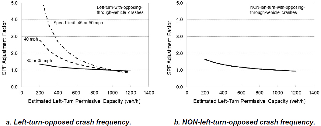
CPM for NON-Left-Turn-Opposed Crash Frequency
This section describes the CPM for predicting nonLT crash frequency (all severities). For each SPF and AF component of the CPM, the description includes one subsection that (a) presents the parameterized equation and (b) includes a figure illustrating equation trends. The CPM (and its SPF and AF components) is described by the following equation.
| Equation 57 |
where,
| Np,nonLT,i = | predicted average nonLT crash frequency during hour i of the typical day for the subject intersection leg (i = 0 to 23) (crashes/yr); |
| Nspf,nonLT,i = | predicted average nonLT crash frequency for base conditions during hour i of the typical day for the subject intersection leg (i = 0 to 23) (crashes/yr); |
| AFlt,nonLT,i = | nonLT SPF adjustment factor for left-turn permissive capacity for hour i; and |
| Cf,nonLT = | nonLT SPF calibration factor. |
This equation is used to evaluate one specified hour for a given signalized intersection leg. The intersection leg of interest must have an opposing left-turn movement that is served by permissive or protected/permissive left-turn operation.
The predicted value from the equation represents the annual average nonLT crash frequency for the specified hour. Multiple hours of the typical day can be evaluated by repeated application of the equation. The predicted average nonLT crash frequency for each hour can be added to estimate the average crash frequency for the combined set of hours.
If the operating conditions being evaluated exist only for a specific subset of the days of the typical week, then the predicted average crash frequency is multiplied by the number of applicable days per week and then divided by 7. For example, if the signal timing plan being evaluated applies only to weekdays (i.e., Monday to Friday), then the analyst would multiply the predicted average crash frequency by 5/7 (= 5 days per weekday/7 days per week).
Safety Performance Function.
The predicted average crash frequency for base conditions is described by the following equation.
| Equation 58 |
Where the AAHTa,i volume variable represents the annual average hourly volume during a specified hour i for the subject intersection leg. The coefficient “-1.075” corresponds to the Year 2023. The calibration factor Cf (to be provided by the analyst) will provide the necessary adjustments to ensure that the model predictions reflect the desired year of application and local conditions.
The SPF relationship between predicted nonLT crash frequency and hourly traffic volume is illustrated in Figure 30b. It is applicable to annual average hourly volumes as large as 1,200 veh/h but may be used with caution to evaluate volumes slightly larger than this value. The trend line indicates that intersection legs with higher volume have more frequent crashes.
Adjustment Factor for Left-Turn Gap Availability.
The AF for left-turn gap availability is described by the following equation.
| Equation 59 |
where, clt,perm,i is the opposing left-turn permissive capacity during hour i (veh/h).
The opposing left-turn permissive capacity variable is computed using Equation 42. The base condition for this AF corresponds to an opposing left-turn capacity of 1,000 veh/h. The AF applies to left-turn permissive capacity in the range of 200 to 1,200 veh/h.
The estimated AF trend for nonLT crash frequency is shown in Figure 31b. The trend line in this figure illustrates the values obtained from Equation 59. The trend indicates that intersection approaches with high left-turn permissive capacity have a slightly lower crash risk than those approaches with a low capacity.


