There is one way in which quantum mechanics has indisputably progressed since the interpretations discussed in Chapter 5 were invented. To understand it, we must prepare to visit a rather strange place that was invented by the mathematician David Hilbert. It is called Hilbert space in his honor.

The key idea is that in a space with a sufficient number of dimensions, a single point can describe the state of an entire system, however large. We’ll start with a simple example. Let’s suppose you own a trucking business that transports goods between New York and Chicago. If you own just one truck and it is always somewhere on the interstate highway between the two cities, you can indicate its position at any given moment by a point on a one-dimensional graph, a straight line, as in Figure 6-1a. The truck is driven by Albert.

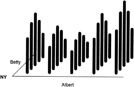
But now let’s suppose that your business expands to two vehicles, with a second truck driven by Betty. You could indicate their positions using two different points on your original graph, by using two different markers. But you could also indicate their positions using a single

point on a two-dimensional graph, as shown in Figure 6-1b, where the horizontal axis gives Albert’s position and the vertical axis Betty’s position. If you got a third vehicle and driver, you would need a three-dimensional graph to keep track of the whole fleet with a single point, as in Figure 6-1c, and so on. Obviously, you will need an n-dimensional graph to keep track of n trucks. You cannot readily visualize a graph of more than three dimensions, of course, but it is perfectly possible to handle mathematically.

If you switch your business to operating a fleet of ships, you will need a graph with two dimensions for each ship, because ships are not confined to roads, and can freely roam a two-dimensional surface; it takes two coordinates per ship to record the latitude and longitude. Aircraft would need three coordinates per vehicle, to include the altitude. To know what orbit a spaceship is going to follow, you need to know not only its position but also its speed in the x, y, and z directions, so it takes a graph of six dimensions to record the full trajectory information for one spaceship. If you have 10 spaceships, your graph needs 60 dimensions, but a single point on it still records all the information about your fleet that you need to know.

Of course what we’re really interested in is not trucks or spaceships but fundamental particles. If the universe consisted of pointlike classical particles, we would need 6N dimensions to keep track of a system of N particles including their positions and speeds: 12 dimensions for a two-particle system, 18 for a three-particle system, and so on. There are perhaps 10⁸⁰ particles in the observable universe, so a single point in a space of about 10⁸¹ dimensions could record the exact state of the entire classical universe. ¹ If that sounds like a lot, just wait….

Quantum systems are more complex than classical ones and require more information to describe them. Suppose you are back to owning just one truck, but it’s a quantum one. Even if it sticks to the route between New York and Chicago, its position is described not by a dot on a line but by some kind of probability wave having a specific value

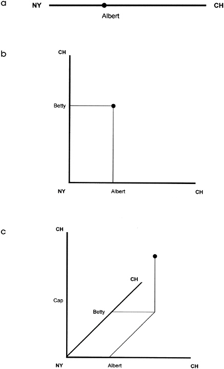
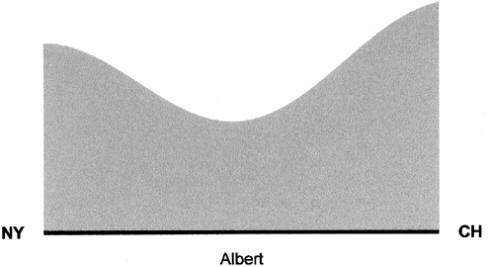
FIGURE 6-2 Albert’s probability wave.

at every point along the route, as shown in Figure 6-2. The shape implies that Albert tends to loiter near the ends of his route.

This is bad news for our project to record all the information about his position in the most compact way possible. To fully record the information in Figure 6-2, we would have to write down the height of the graph at every point along the x axis; an infinity of points, so an infinity of values. Things get more manageable if we only need to know roughly where Albert is: say, in which county out of 5 counties along the route. Then we get a bar chart as shown in Figure 6-3a. The information is given in the height of 5 individual bars, 5 numerical values, and we could record it by placing a dot at an appropriate position in a space of 5 dimensions. If we add a second truck, driven by Betty, her graph might look like that in Figure 6-3b, and we could record the position information for both trucks by a point in a 10-dimensional space. This is worse—in the sense of more extravagant—than the situation for classical trucks or particles, but not that much worse, for the basic rule is still additive. A two-particle system will require a space of twice as many dimensions to describe it as a one-particle system.

For display purposes, you could combine the information on both the graphs into a single 3-dimensional graph, as in Figure 6-3c. How-

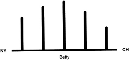
FIGURE 6-3b Probability of Betty being found in each location.

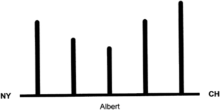
FIGURE 6-3a Probability of Albert being found in each location.

ever, at the moment, Figure 6-3c does not contain any more information than 6-3a plus 6-3b. Although it has 25 columns, a point in 10-dimensional space still contains all the information we need to generate it.

But now let’s introduce Albert to Betty. The results are dramatic. They start to interact; indeed, they fall in love and get married. It’s all very sweet, but now the interaction makes the probability wave describing where your trucks are much more complicated, as shown in Figure 6-3d. For example, in many places the probability that Albert

and Betty will be close together is high, but for some reason Albert tends to avoid Cleveland, where his mother-in-law lives, when Betty is there. The point of the story is that once Albert and Betty have started to interact, the probability wave describing them can no longer be decomposed into two simple Figures like 6-3a and 6-3b: Figure 6-3d simply contains too much information. There are 25 independent columns, so it would now require a point in a space of 25 dimensions to record the information.

The general rule is that when we join two classical systems and allow them to interact, we just add the number of dimensions of the two originals; but when we join two quantum systems, we must multiply the number of dimensions of the originals. The Hilbert space of a system containing even a few particles has a mind-boggling number of dimensions.

What is the significance of Hilbert space? Hilbert space represents a quantum system before it is measured. When we do a measurement, the space will collapse to a specific state represented by a single point (as when we ring Albert and Betty on their cell phones and discover their actual positions). But before a measurement is made, we can think of Hilbert space as being filled with a kind of grey mist whose density at each point corresponds to the probability that the system will collapse to that particular set of values. This mist turns out to be highly amenable to mathematical analysis: it slops around following very simple rules, in fact even simpler than those that govern the behavior of a real fluid like water. So, despite the large number of dimensions involved, the best way to calculate the evolution of an isolated quantum system is to use Hilbert space.

Now you understand the dilemma of mathematical physicists dealing with quantum. The rules of quantum are beautifully simple. But all except the simplest quantum processes—for example, those of tiny isolated systems such as the hydrogen atom—happen in a space of such a colossal number of dimensions that it becomes impossible to simulate them on the most powerful computers now available, and utterly hopeless to try to visualize them with our own minds.

Hilbert space is usually described as totally abstract, utterly remote from the three-dimensional world of our ordinary perceptions. But there is a well-known experiment that calls for creating a large bubble of Hilbert space, embedded within the everyday world, which you could in principle touch. We have encountered it already. I am talking about Schrödinger’s famous cat.

To really do Schrödinger’s famous cat experiment, we would need to create a cat box that no information could leak out of, a box of macroscopic size that was truly and utterly sealed from the outside world. Just for fun, let us see if we could conceivably do this with present or near-future technology. In the interests of both scientific progress and cat welfare, we will replace the cat with a human observer, a kind of philosopher-astronaut.

It is vital that the box does not touch anything, so we will start by going into space where it can be allowed to float free in microgravity without any connecting struts. To shield against the high-energy charged particles called cosmic rays, which are found everywhere in space, we will hollow out a chamber at the center of some natural object, an asteroid or comet nucleus. We must then protect the central chamber against particles caused by radioactive decay of elements in the asteroid, probably with a thick shield of pure metal. I cannot resist telling you an odd fact at this point. Since the first atomic tests in the 1940s, all the steel made on Earth has been slightly contaminated with radioactive particles present in the atmosphere, which inevitably get into the blast furnace because large amounts of air are needed for combustion. When scientists need steel that is completely free of decaying radioactive nuclei, they get it from a surprising source. After World War I, the German battleship fleet was scuttled at Scapa Flow in Scotland, the giant natural harbor where the British Grand Fleet used to be based. When nonradioactive steel is required, scuba divers go down and carve chunks of pre-Atomic-age steel from the battleships, which thankfully provide a huge resource of the material. Within the asteroid, we will construct a thick sphere of this ultrapure steel.

The cat box, or philosopher box as it is now, floats within this

central shield, and within it is a further thin spherical shell like a Christmas bauble that is cooled to the lowest temperature practicable, in the milli- or perhaps even micro-Kelvin range, to suppress the radiation of infrared photons. The inner shell contains a perfect vacuum except for the very occasional very low energy infrared photon emitted by the walls. Because such photons have a wavelength of several meters, they reveal nothing about the position or state of the central chamber beyond the fact that it is there.

In theory, the space capsule now no longer contains a philosopher-astronaut, but a Hilbert space, a probability distribution of philosopher-astronauts doing increasingly divergent things, as their personal histories diverge depending on exactly how many photons hit each cell of their retinas and other quantum events that multiply into macroscopic consequences in various ways. If we could look inside the capsule (which is, by definition, impossible), we might imagine seeing something like a multiple-exposure photograph. Is the astronaut writing, or brushing her teeth, or just staring into space? This is the image that inspired the title of this book. Rabbits are famous for their tendency to multiply; what a Schrödinger box really contains is not one of what we originally put in it, but many.

We have seemingly created a macroscopic bubble of Hilbert space, in which different probability histories of the astronaut, eventually diverging quite significantly, can trace themselves out. In principle, we could do a test to prove that this has happened, using interference between the different histories, and we will return to this possibility in the last chapter. However, when the capsule is opened the astronaut herself will report nothing out of the ordinary—the Hilbert space will instantly collapse to a single point, selecting just one of all the possible states that it has been exploring.

Alas, there is at least one effect that might still make this experiment impossible, despite all our elaborate precautions. One effect that we do not know how to shield against is gravity. Although the center of the capsule will automatically remain in the same position no matter how the astronaut moves about, only a perfectly symmetrical object can have a perfectly spherical gravitational field. A real object—like Earth or a space capsule with an astronaut in it—has a

field with subtle variations betraying information about the internal disposition of its mass. Remember Borel’s thought experiment in which shifting a small rock light-years away could change the positions of air molecules in Earth’s atmosphere, via gravitational effects amplified with every molecular collision? It is difficult to calculate the extent to which such effects would continuously measure the capsule in the above experiment, but it might well be sufficient to make the macroscopic superposition we are trying for impossible.

The analysis of Hilbert space has thrown an extraordinary new light on the process we call quantum collapse. In 1970, Dieter Zeh at the University of Heidelberg demonstrated something remarkable. In a system that evolves in Hilbert space, whose components interact significantly, the mathematics predicts that although at first sight things appear to proceed quite unselectively—there is no telling, for example, what position one particular particle is likely to occupy—patterns nevertheless start to emerge that are durable in the sense that they continue to be strongly affected by patterns of high co-probability, but in a rapidly decreasing fashion by patterns of low co-probability. The mathematical process by which inconsistent patterns exert increasingly small effects on one another is called decoherence.

Decoherence can effectively explain quantum collapse—or at least apparent quantum collapse. To see how, let us consider a nested system of Schrödinger’s cats. Assume that the astronaut described above takes into the capsule with her a small cat box designed on the same lines, with Schrödinger’s original diabolical arrangement that might kill the cat with 50 percent probability.

We seal the capsule. From our point of view, both the astronaut and the cat are in Hilbert space. But we know that after a certain time, she will open the box. What does the Hilbert space model now reveal? It tells us that as soon as she starts to open the cat box, the possible states of herself very rapidly become entangled with those of the cat. There are states of her that are rejoicing, having found a live cat, and states of her that are mourning, having found a dead one. But these

different states very rapidly cease to have a significant effect on one another. Each state of her has apparently seen a quantum collapse in which the cat has become definitely dead, or definitely alive.

At this point it is really impossible to avoid a mention of many-worlds because: What happens when you open the astronaut’s capsule? You are going to see either a happy woman with a living cat in her arms, or a sad woman holding a dead one. If you accept that the Hilbert space analysis applies to the whole universe, then what is really happening is that one version of you is becoming correlated with the happy-live-cat outcome, and another version of you with the sad-dead-cat one.

We will have more to say about this later, but I am certainly not yet claiming that this is a proof of many-worlds. A single-worlder might describe the opening of a Schrödinger’s cat box something like this:

“When I opened the box, the outside environment started to measure what was in there. The very first measurement photon out of the box might give a strong clue—for example, if it was an infrared photon at the temperature of a live cat.

“Just as when you scratched one lottery card, it made a certain outcome of scratching the other more likely, so a measurement consistent with (say) a living cat makes subsequent measurements consistent with that outcome more likely. And so either a live cat or a dead one emerges, rather than some gruesome combination. From the abstract processes of Hilbert space, consecutive measurements brought a specific consistent reality into being.”

The single-worlder might have a point. Despite my simplified account above, it remains controversial whether you can in fact get sensible numbers out of Hilbert space without some form of context dependence—some privileged starting point such as a unique reality from which you can measure everything. But we will postpone this argument to a later chapter, and concentrate for now on the solid achievements of decoherence.

Decoherence theory allows us to calculate exactly the timescale over which any given system will decohere—in the old language, the time for quantum collapse to happen. I am not going to describe the math, but it is useful to get some idea of how long collapse is predicted to take in certain situations. One sort involves the spatial localization of small objects whose position is measured from time to time by interactions in which they scatter photons and other particles in their vicinity. Table 6-1 is adapted from a paper by Erich Joos.²

The top left figure in this table tells you, for example, that a particle of dust a hundredth of a millimeter across (just big enough to be visible with a strong magnifying glass) that is floating in interstellar space, and whose position has become uncertain by a centimeter, is likely to pop to a relatively precise location in about a microsecond. However, if its position is uncertain to only about the same distance as its own diameter, a hundredth of a millimeter, it will take a second or so to get relocalized. Note the huge variation from the top right to the bottom left of the table. Relocalization becomes much faster as you approach Earthlike conditions of temperature and atmospheric pressure. It also gets much faster for larger objects. There is probably nowhere in the natural universe where objects larger than dust grains are delocalized to any significant degree, because the famous 3^o Kelvin

cosmic microwave background radiation, remnant of the Big Bang, is all-pervasive.

There are subtler forms of decoherence than simple localization, however. Another system of interest is a regular oscillator whose motion is slowly decaying, like a swinging pendulum subject to friction. It turns out that the decoherence time of such a system is directly related to the damping time—that is, the time it takes for the pendulum’s swing to decrease to half its original value. This link between quantum decoherence and the increase of classical entropy, the slowing of things due to friction, is a tremendously important theoretical result. Unfortunately for anyone hoping to witness a pendulum in a superposition of different angles of its swing (an effect you can sometimes see in trick photographs), the ratio of the decoherence time to the decay time is extremely small, of the order of 10⁴⁰ in the case of a 1-gram pendulum on Earth.

However, this ratio is proportional to the absolute temperature of the surroundings, and to the mass of the object. It gets more reasonable for a small object spinning in a vacuum, an object for which the damping time is also extremely long, because there are only tiny effects tending to slow the spin. Such an object can remain in a superposition of different angular positions for an appreciable time, but again, naturally occurring examples are spinning dust particles in interstellar space rather than large terrestrial objects.

Let us now return to Earth, however, and emphasize that decoherence is not just a theory. It can be tested in doable experiments. Such tests have already been performed by the redoubtable experimenter, Anton Zeilinger of the University of Vienna, with interference experiments using relatively large objects—fullerenes, football-shaped molecules whose basic form is a cage of 60 carbon atoms.

Zeilinger looked at ways in which environmental decoherence—that is, the environment “reading” the position of the molecules—tends to degrade the interference pattern obtained in a two-slit experiment. One such test involved doing the experiment in a space

that was not a perfect vacuum, so that occasional collisions with gas molecules caused decoherence, degrading the interference pattern. Another used molecules that were hot enough to emit infrared photons as they flew along their trajectories, giving away information about their positions.

In both experiments, the predictions of decoherence were confirmed. The error bars were relatively large, but new experiments now being proposed should dramatically increase the accuracy. Indeed, as we’ll see in a later chapter, devices like quantum computers, which are extremely sensitive to the effects of decoherence, naturally provide a way of measuring it to very high accuracy, and that is part of the motivation for trying to build such devices.

Unless something very unexpected emerges, the mystery of where, when, and how quantum collapse occurs must be considered solved. It is, quite simply, decoherence that does it. Dieter Zeh’s hypothesis has been confirmed by 30 years of calculation and experiment, and it is something of an indictment of the system by which scientific advance is recognized and popularized that this tremendous progress is not better known.

There was one point about Hilbert space that I rather skated over: the fact that strictly speaking, the probability wave associated with even a single particle needs a Hilbert space of infinite dimensions to describe its exact value everywhere. If you have a good physicist’s distaste for infinities, let me throw you a lifeline—in fact, two lifelines.

First, there is nowadays strong evidence from the field of general relativity that the maximum amount of information that can be stored in and retrieved from a finite-volume region of our three-dimensional universe is itself finite. There is even a formula for calculating it, called the Bekenstein limit after its discoverer. No one knows yet quite what implications this has for Hilbert space descriptions of the universe. There have always been awkward clashes between general relativity and quantum theory. But it is possible that it means that the number of dimensions required for Hilbert space is not quite infinite, merely

mind-bogglingly colossal (still much larger than the mere 10⁸¹ dimensions or so required to describe a classical universe). So, wherever I have used the word “infinite” in connection with Hilbert space dimensions, you can possibly substitute “vast.” The implications might be important, but this is a very controversial area that we will return to in the final chapter.

Be that as it may, there is one aspect of most kinds of particles that requires not an infinity, or even a mind-boggling number, of dimensions of Hilbert space to describe it, but exactly two. As well as having a position, many particles have a much simpler intrinsic property, called spin in the case of electrons and polarization in the case of photons. Spin and polarization represent internal properties of particles. In terms of our trucker analogy, they might represent something like the angle at which the driver’s cigarette is currently pointing. (I regret to tell you that Albert and Betty are both chain-smokers.)

External quantum properties like position along the x axis must be represented by a waveform containing an infinity of real numbers, giving the probability of the particle being found at each possible point along the axis. After collapse, the result of a measurement is a single real number which still requires an infinity of digits to record its exact value, like 119.3564218…. The universe “knows” an infinity of real numbers, and gives you one back. But a quantum value such as polarization can be represented by just two real numbers—like the direction in which Albert’s cigarette is currently pointing, given in terms of compass bearing and elevation—and when you collapse it, you get back just one single binary digit, a yes-or-no answer, as if all you can record from outside the truck is whether Albert ultimately discards the cigarette stub out the right- or left-side window.

The two real numbers describing spin could be drawn rather unimaginatively in a bar-chart with only two columns, but a neater way is shown in Figure 6-4, called the Bloch sphere after its inventor. Here the direction of the particle’s spin axis (the direction Albert’s cigarette is pointing) is shown as the latitude and longitude of a point on an imaginary sphere. On measurement, the vector shoots to either the north or south pole.

It was David Bohm who first realized that, in a less-is-more kind of way, using these modest internal quantum properties might yield

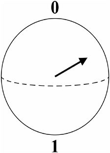
FIGURE 6-4 Bloch sphere.

the most practical way to perform the kind of test of quantum nonlocality that we met in the Bell-Aspect experiment, far more doable than the experiment originally proposed by Einstein. Later, David Deutsch and others realized that harnessing these internal quantum values is also the way to a viable quantum computer. Before measurement, the uncollapsed vector shown in Figure 6-4 can be thought of as a qubit, the quantum equivalent of a binary digit; when it is collapsed by measurement, it becomes an ordinary bit, by assigning the values 0 and 1 to the north and south poles in the diagram. For more on quantum computers, see Chapter 11.

The arena of Hilbert space, and the process of decoherence, have given us deep insights into quantum that the pioneers who invented the old interpretations did not have. But the new concepts do not by themselves answer the key interpretational puzzles of our PPQs and they do not help us to visualize the processes of quantum in terms of the space and time we are familiar with, to tell ourselves a meaningful story of what is going on.

Indeed, the relationship between Hilbert space and real space conceals rather than explains perhaps the most troubling feature of quantum, its nonlocality. Sometimes things that happen in a smooth, orderly way in Hilbert space, as the gray shading develops in its fluidlike way, can correspond to rather startling goings-on in ordinary space. We have already met the EPR paradox, which arises because two photons widely separated in ordinary space can share the same small Hilbert space. There is another quantum phenomenon that can give rise to apparently faster-than-light effects.

Most people have heard of quantum tunneling. Suppose that you fire a particle such as a photon or an electron at some kind of wall that it doesn’t have enough energy to penetrate. The wall can be an actual physical barrier, such as a thin sheet of aluminium, or a more subtle energy barrier, the equivalent of a hill that the particle does not have sufficient energy to roll up and over. Under these circumstances, the rules of quantum mechanics—specifically, the Heisenberg uncertainty principle—predict that because the probability wave associated with the particle slops over beyond the wall, occasionally the particle will appear to tunnel straight through what would otherwise be an impassable obstacle, just by happening to jump from one part of its probability wave to another.

A disturbing feature of quantum tunneling is that it appears to happen instantly. We can describe this in words: “Any time that you choose to measure the particle, you will find that it is on one side of the wall or the other. The implication is that at some point, it must have moved across the wall in no time at all.”

Those are just words. But the mathematics does also seem to describe the particle leaping across the wall instantly, and when you watch a computer simulation of the probability wave associated with the particle, the central part describing where the particle is most likely to be detected does indeed seem to proceed faster than light. The matter is unclear enough that experimental physicists, including highly respected ones, have run tests to see whether they can transmit data faster than light using quantum tunneling, and some even claim to have succeeded.

Now, before anyone gets too excited, I hasten to add that you almost certainly can’t do this. More careful work, both in computer simulations and with actual photons, indicates that although the probability waves do seem to travel faster than light at certain points, you cannot propagate a disturbance along them at this speed. You cannot really send information faster than light, with the paradoxes that could imply. My point is that a good visualization or interpretation of quantum should not even tempt us to think such a thing could happen. Hilbert space is a good place to do math, but it does not provide us with a clear intuitive picture of what is going on in the three-dimensional world.