Review of the Long-Term Operations of the Central Valley Project and the State Water Project (2026)
Chapter: 3 Old and Middle River Flow Management
3
Old and Middle River Flow Management
The Committee was charged with assessing the state of science for Old and Middle River (OMR) flow management and recommending ways that modeling and monitoring strategies and decision support tools can be changed, improved, or replaced to more accurately assess the impacts of OMR flow management. This chapter first describes the OMR Flow Management Action, including the specific actions taken during a typical wet and dry OMR season and the thresholds that, if crossed, lead to constraints on exports. It also assesses whether existing OMR management practices are grounded in reasonable scientific concepts, whether existing scientific information supports those concepts, and how better information might be obtained.
The chapter makes three primary points. First, existing OMR flow management, which uses takes at the pumps, flow levels, and turbidity levels as triggers for limitations on pumping, does have a reasonable scientific basis, although significant uncertainties exist about how well each trigger correlates with fish protection. Second, because of those uncertainties, OMR management could be improved, though such improvements would require changes to monitoring and modeling approaches. Third, the most promising changes would involve, first, more robust monitoring to better assess fish abundances, distributions, and movements within the Delta and, second, the application of a Delta-wide hydrodynamic model that enables mapping of the spatial and temporal influence of pumps. With these advances, water managers could move beyond management strategies that focus primarily on takes at the pumps.
OLD AND MIDDLE RIVER DESCRIPTION
The Central Valley Project (CVP) and the State Water Project (SWP) (sometimes referred to collectively as the Projects) divert enormous quantities of freshwater from the San Joaquin and Sacramento rivers, with some of the largest diversions taking place through the south-Delta pumps. The Projects deliver water from those pumps to contractors, primarily in the San Joaquin Valley and Southern California. The C. W. “Bill” Jones Pumping Plant (the Jones pumping plant), operated by the San Luis & Delta-Mendota Water Authority for the U.S. Bureau of Reclamation (USBR), generally limits maximum pumping to 4,600 cubic feet per second (cfs) due to subsidence in the Delta-Mendota canal (USBR, 2024a); otherwise, the pumping capacity could be 5,200 cfs. The Harvey O. Banks Pumping Plant (Banks pumping plant), operated by the California Department of Water Resources (CDWR), has a capacity of 10,300 cfs (CDWR, 2024a). Figure 3-1 shows the generalized, highly simplified flow paths cre-
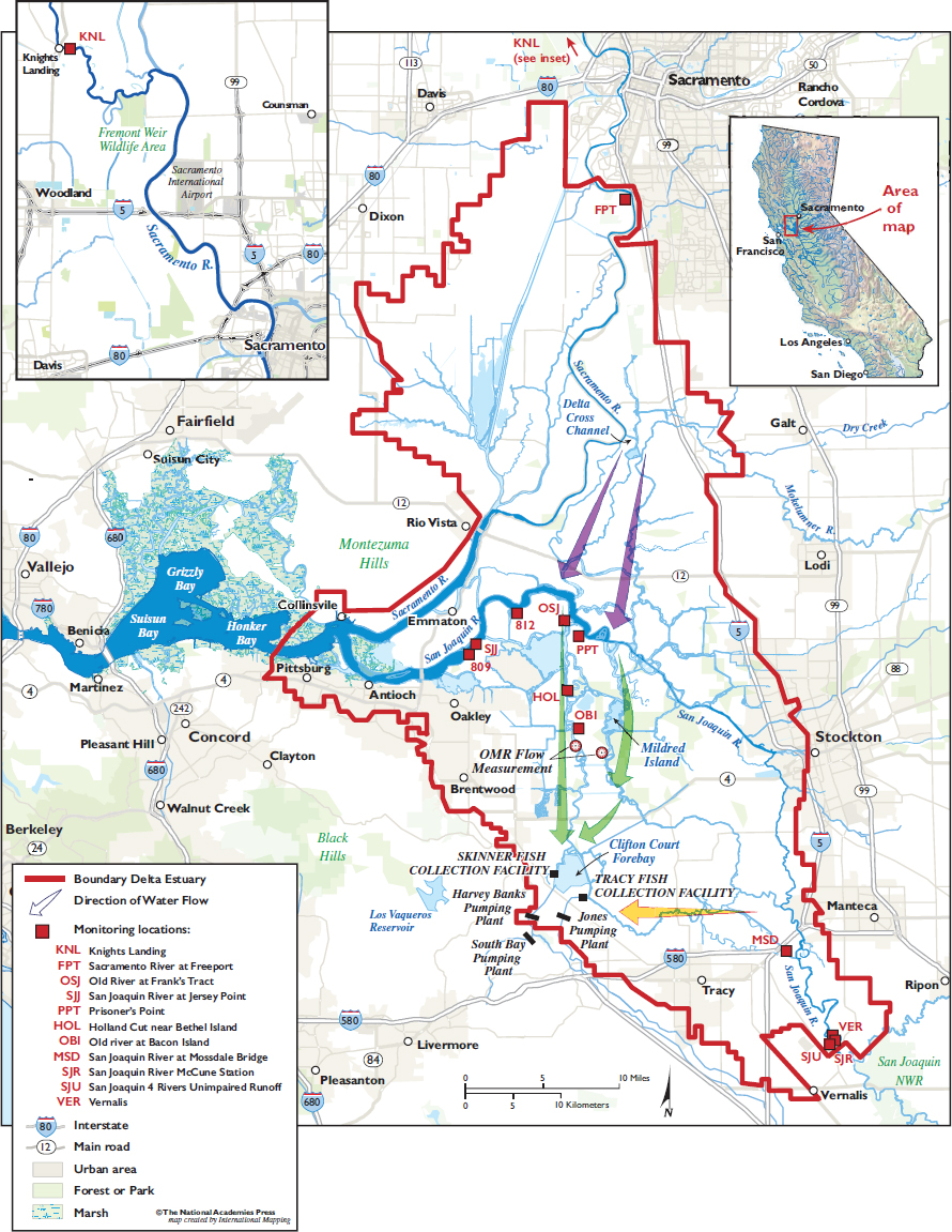
NOTE: Purple arrows indicate direction of water flow when the Delta Cross Channel is open, while green and yellow arrows indicate direction of water flow from the Sacramento and San Joaquin rivers, respectively, when the pumps are running.
SOURCE: Kevin Lear, International Mapping Associates.
ated by opening of the Delta Cross Channel (DCC) and operation of the pumps, promoting water flow away from the Sacramento and San Joaquin river channels and toward the South Delta.
OMR flow management occurs in a highly complex, tidally affected inland delta. Freshwater inputs to the OMR reaches of the Delta are primarily from the Sacramento and San Joaquin rivers (about 75 and 25 percent of inflow, respectively), both of which are regulated by upstream dams. However, semi-diurnal mixed tides also affect flow in the OMR reaches, with effects dependent on tidal phase, meteorological conditions, and freshwater inflows. Saltwater (greater than 2 parts per thousand [ppt]) can intrude into the Delta, depending on tides and freshwater flows, and water quality standards are designed to prevent salt from degrading the quality of exported water.
Adding to these challenges is the need to protect the six listed fish species that both pumping facilities can directly entrain, meaning the fish are drawn into water intakes for the pumps. Exports can also cause fish to become trapped in the OMR corridor or in Clifton Court Forebay prior to reaching the Banks pumping plant, thereby failing to complete their natural migration and becoming increasingly subject to predation (ESA, 2018; NOAA, 2013). Other more indirect impacts to fish occur across the Delta because pumping changes the flow patterns within channels, sometimes rerouting fish to places where habitat conditions are poorer (NMFS, 2024, Section 7.5). Both direct and indirect effects of pumping cause fish mortality. Salvage of entrained fish occurs at both pumping plants, and the salvaged fish are trucked to one of six locations near the confluence of the Sacramento and San Joaquin rivers.
The objectives of OMR flow management are to ensure that water delivery obligations are met while minimizing the negative effects of exports on protected fish species (NMFS, 2019, p. 476). Over the years, the U.S. Fish and Wildlife Service (USFWS) and the National Marine Fisheries Service (NMFS) biological opinions have set forth specific steps to meet these broader goals. The OMR Flow Management Action began in 2009 as part of those biological opinions, with pumping rates reduced in accordance with constraints imposed by the federal and state Endangered Species Acts (ESAs), and the action has continued to be part of subsequent biological opinions. A primary means by which USBR and CDWR comply with the biological opinions is by managing tidally averaged flows in the OMR corridor just north of the pumps (so-called OMR flow). These flows can range from -12,000 to 13,000 cfs in each channel near the two OMR flow measurement sites (Figure 3-1), where negative flow indicates net flow to the south. Without pumping, both positive (downstream) and negative (reverse) flows would be expected to occur over the course of a day in the channels during ebb and flood tides, respectively, with the net daily flow being positive. Depending on the time of year, CVP and SWP exports can result in a negative net daily (reverse) flow in portions of these channels. OMR flow management regulates the amount of freshwater pumped by the Jones and Banks pumping plants during a period that generally extends from December through June, which is the period when sensitive life stages of the listed fish species are found in the Delta (Figure 3-2).
The biological opinions that govern OMR flow management are part of a broader set of laws and physical constraints that affect pumping levels. The general conditions and legal constraints—including but not limited to biological opinions—that limit exports during the period of OMR flow management are listed below1:
- Infrastructure capacity: The reservoirs, pumps, and canals have capacity limits, and sometimes these limits control the pumping levels.2
- Water quality and flow standards, of which there are dozens,3 as outlined in Water Rights Decision D-16414 (State Water Resources Control Board, 2019).
___________________
1Not every possible constraint is listed; rather, the focus is on those constraints highlighted by USBR and CDWR as central to OMR flow management at the Committee’s Meeting 2. For example, the list does not mention constraints stemming from the voluntary agreements, such as limiting exports to half of the San Joaquin River inflow (Hutton, 2008), which, even in wet years, can be low due to substantial diversions in that basin.
2For example, in some wet years pumping is curtailed when the San Luis Reservoir is full, as there is no place to put the water.
3See https://www.waterboards.ca.gov/waterrights/water_issues/programs/bay_delta/deltaflow/docs/closing_comments/dwr_closing_attachment.pdf.
4See https://cawaterlibrary.net/document/water-rights-decision-1641-d-1641/.

NOTE: Fall-run and late-fall-run Chinook are not ESA-listed species. Sturgeon is not included in the graphic.
SOURCE: Schreier et al. (2024).
- Biological opinions from USFWS and NMFS: The 2024 biological opinions restrict 14-day running averaged OMR flow to values between -2,000 and -5,0005 cfs to reduce entrainment of smelt and salmonids.
- Incidental take permit (ITP) from the California Department of Fish and Wildlife (CDFW) for longfin smelt, Delta smelt, and spring-run and winter-run Chinook salmon: The ITP restricts OMR flows to values between -1,250 and -5,000 cfs.
- The need for a minimum export of 1,500 cfs to meet health and safety needs.
- Contractual obligations for Project water: The highest priorities are senior water right holders and wildlife refuges (see Appendix B), and delivery to those right holders may limit the amounts of water flowing into the Delta, thus reducing the amount of water available for export.
- Storm-flex, which allows exports to exceed normal thresholds during storm conditions in the Delta, (e.g., allowing the 14-day average OMR flow to reach -6,250 cfs under certain criteria) (USBR, 2024b, pp. 3-66 to 3-67).
- Emergency drought operations (e.g., California Water Boards, 2016, and Temporary Urgency Change Orders).6
Of the aforementioned constraints, a primary control is D-1641, which defines water quality conditions that must be met at different parts of the Delta and establishes constraints designed to make sure those conditions are attained. Hence, D-1641’s requirements govern Delta outflows, salinity levels, and export-to-inflow ratios. D-1641 also establishes a framework for adjusting these requirements. The decision specifies automatic relaxations, which are tied to water-year type; those relaxations derive from a recognition that some water quality objectives may be too difficult to attain in dry or critically dry years. CDWR and USBR also may file Temporary Urgency Change Petitions with the State Water Resources Control Board, which may grant those petitions through Temporary Use Change Orders (TUCOs), which can allow short-term modifications to D-1641 requirements beyond the automatic water-year-type relaxations. TUCOs typically include measures like reduced outflow requirements, movement of compliance points further upstream, and adjustments to export restrictions—especially in dry years.
The particular condition and/or legal requirement that ultimately controls exports depends on the water-year type and the time of year, and it can vary from week to week. The importance of D-1641 as a constraint in wet
___________________
5The -5,000 cfs baseline for OMR flow is based on Grimaldo et al. (2009), which suggested an increase in Delta smelt salvage at OMR flows more negative than -5,000 cfs.
6See https://www.waterboards.ca.gov/drought/tucp/docs/2016cpmarnovadd1_update.pdf.
versus dry years is shown in Figure 3-3. In late 2021, a dry fall meant that D-1641 standards, likely for salinity, were controlling exports. Around January 1, 2022, a “first flush” trigger caused by a storm event (labeled “OMR” in Figure 3-3 and described below) became controlling. However, overall dry conditions that winter led to a return to D-1641 standards as the overall controlling factor for the remainder of the OMR flow management period. In contrast, in late 2022 a dry fall again preceded the OMR flow management period, and D-1641 controlled exports. However, December 2022 storms ushered in a very wet winter, which led to a different set of controlling factors in 2023, including infrastructure capacity, that varied throughout the OMR season.

NOTE: There is a difference in scales on the y-axis.
SOURCE: Schreier et al. (2024).
Actions in an OMR Season
The three main phases of OMR management—onset, duration, and offramp—are described below.
OMR Onset
The 2024 Record of Decision (ROD) for the Long-Term Operation of the Central Valley Project and State Water Project (USBR, 2024c) governs the actions that constitute OMR flow management, including onset. The first condition that controls onset, which can start on or after December 1, is called “first flush.” First flush is defined as when the running three-day average of the daily flow at Freeport (8 miles south of Sacramento on the Sacramento River) is greater than or equal to 25,000 cfs and when the running three-day average of daily turbidity at Freeport is greater than or equal to 50 Formazin Nephelometric Units (FNU).7 During first flush, listed fish are more likely to be moving through the system, and entraining these fish is undesirable, hence the onramping of OMR flow management during such conditions. The second condition that controls onset is the salvage of adult longfin smelt (Adult Longfin Smelt Entrainment Protection Action) or crossing a turbidity threshold indicative of adult Delta smelt entrainment (Adult Delta Smelt Entrainment Protection Action). If none of those conditions is met, OMR flow management automatically starts January 1.
Actions During the OMR Season
OMR flow management during the December–June period is layered and imposes a variety of constraints on exports. The constraints can stem from water quality conditions that occur during the management season or the presence of fish in the Delta. For example, “turbidity bridge avoidance” refers to reducing exports to maintain daily average turbidity to be below 12 FNU at three water quality monitoring stations (OBI, HOL, and OSJ—Figure 3-1). The rationale behind this control is that a continuous area of turbid waters from the San Joaquin River Shipping Channel to the south Delta fish facilities could attract pre-spawning adult Delta smelt to the pumps (Brown et al., 2024). When it is controlling exports, turbidity bridge avoidance restricts the OMR Index (OMRI)8 to no more negative than -3,500 cfs.
Constraints on exports are also imposed if certain environmental or biological thresholds that might indicate entrainment are breached during the management season. Environmental triggers used as surrogates for smelt protection include temperature, turbidity, and Secchi depth, each of which is measured at various locations in the Delta. Biological triggers include a certain number of listed fish salvaged at the pumps, specifically larval, juvenile, and adult Delta smelt and longfin smelt; winter- and spring-run Chinook salmon; and steelhead. Depending on which fish and life stage have been detected above a trigger, and at what time during the season (and only when the ITP or the biological opinions are controlling), OMR flows cannot be more negative than a certain value, which ranges between -5,000 and -2,500 cfs. For example, if the natural winter-run Chinook loss in salvage exceeds some percentage of the Juvenile Production Estimate (JPE), then exports must operate to achieve an OMR flow of no more negative than -3,500 cfs for seven consecutive days. As another example, if salvage of adult longfin smelt exceeds a threshold based on prior months’ San Francisco Bay Study index, exports must be reduced to maintain a seven-day average OMR flow no more negative than -3,500 cfs. The specific triggers that are compared to environmental and fish salvage data are presented in Table 3-1 and discussed subsequently in greater detail.
___________________
7Turbidity can be measured using metrics of FNU or Nephelometric Turbidity Units (NTU). Instream turbidity is typically measured by equipment that uses FNU based on infrared or monochrome light source, while most laboratory equipment uses NTU measured with white or broadband light (https://pubs.usgs.gov/sir/2007/5178/section4.html).
8OMRI is defined subsequently and is similar to flow in the OMR corridor.
OMR Offramp
According to the 2024 ROD (USBR, 2024c), the OMR management period will end prior to June 30 (1) for smelt when water temperature at Clifton Court Forebay exceeds 77°F (25°C) for three consecutive days and (2) for salmonids when daily mean water temperature at Mossdale and Prisoner’s Point exceeds 72oF (22.2°C) for any seven days in June. If temperature cutoffs have not occurred, OMR management ends on June 30.
Other Components of OMR
Calculation of OMR Flows
OMR flows are quantified as the sum of daily averaged tidally filtered flow at two U.S. Geological Survey (USGS) monitoring stations. USGS operates gages on both the Old (station ID 1313405) and Middle (station ID 11312676) rivers, where velocity and water level are measured. These observations are then converted to flow based on a rating curve. Because flows in the OMR corridor are tidally affected, USGS provides a net flow at each site through the application of a Godin filter to the hourly observations; this is standard practice for calculating net flow at tidally affected sites (Walters and Heston, 1982). However, the Godin filter requires 72 hours of observations beyond the current time to estimate a flow and does not perform well when wind and atmospheric pressure changes affect water levels and the direction and magnitude of flow.
Because of the limitations of the time-delayed Godin-filtered net flows, CDWR proposed the use of an OMRI for OMR management. Conceptually, the OMRI is a water balance using measured riverine inflows, measured exports by water projects and estimates of other diversions, channel depletions, and precipitation (CDWR, 2017; Hutton, 2008; Sandhu et al., 2016).9 An analysis by CDWR (2017) demonstrated a very close correlation between the USGS tidally filtered measured flows and the OMRI over long averaging periods; the correlation was higher for wetter years compared to drier years. (For an example of OMR flow and OMRI, see the gray and green lines in Figure 3-3, which also shows intervening missing periods of tidally filtered flow filled in by the OMRI.) CDWR recognizes the need for additional work to help close the water balance, including additional instrumentation, improved estimates of consumptive water use and evapotranspiration (ET), and a better understanding of groundwater and channel depletion (CDWR, 2017). Nevertheless, the OMRI is the flow metric currently used for management.
Delta Cross Channel
The DCC is a controlled diversion channel between the Sacramento River and Snodgrass Slough, north of the Delta. Operation of the DCC is part of OMR flow management because the DCC improves the efficiency of conveying water from the Sacramento River to both export facilities. By moving water from the Sacramento River to pumping plants, opening the DCC can improve water quality in the central and southern Delta and reduce salinity intrusion from the west. The gates are closed to protect outmigrating Sacramento River salmonids from entering the interior Delta where mortality is expected to be high. Fish monitoring data from Knights Landing and Sacramento are used to determine the presence of juvenile salmonids that may enter the Delta (USBR, 2023). In addition, whenever flows in the Sacramento River at Sacramento reach a sustained flow of 20,000 to 25,000 cfs, the gates are closed to reduce potential scouring and flooding that might occur in the channels on the downstream side of the gates (USBR, 2021). Between December 1 and January 31, the DCC gates are closed unless there is a risk of exceeding water quality standards. For the bulk of the OMR flow management season (February 1–May 20), the DCC gates are closed. From May 21 to June 15, the DCC gates are closed for 14 days (generally weekdays to accommodate recreation on the weekends), after which time the gates open permanently until fall.
___________________
9See https://www.cbr.washington.edu/sacramento/data/metadata/method_omr.html.
Decision Making During OMR Management
Major decisions about OMR flow management are made by the Water Operations Management Team (WOMT) on a weekly basis (Table 1-1). The WOMT considers summaries of water operations, operational outlooks, and notes provided by other participating teams, including the Salmon Monitoring Team (SaMT) and Smelt Monitoring Team. These teams consider a myriad of factors such as data on hydrology, flow requirements of the ITP and biological opinions to meet specific water quality and entrainment criteria, water quality (salinity, temperature, Secchi depth/turbidity at specific locations), and smelt and salmonid presence and fish distribution. The WOMT also receives input from the Delta Monitoring Workgroup, which consists of water contractors and other stakeholders. In all, export decisions consider regulatory constraints, risk assessments, historic and real-time data, and model outputs from water quality experts, biologists, water contractors, and operators. Many of the data sets about current conditions on Delta smelt, operational data, onset and offramp conditions, and other metrics relevant to OMR management are compiled and visualized daily at the SacPas website.10 If the WOMT cannot agree on a path forward, the issues elevate to agency directors. Decisions to change the export rate can take several days to implement due to CDWR/USBR administrative protocols for coordinated operations, facility (e.g., pumps, gates) adjustments and reaction times, and other factors.
Table 3-1, compiled by the Committee from multiple documents, lists the many hydrologic, water quality, and biological triggers that currently play a role in OMR flow management, organized by management phase. For each trigger, Table 3-1 shows the location of the measured parameter, the threshold value(s) of the measured parameter, and the operational consequence of exceeding the threshold. Since implementation of the 2024 ROD, these triggers and their corresponding thresholds have taken on greater importance in OMR flow management because other criteria that used to be part of OMR flow management, such as estimating the percentage of salmonid populations affected by a change in export rate, have been removed from the decision-making process. Now, decisions about changing the export rate (when the biological opinions or the ITP are “controlling”) are almost entirely based on the exceedance of such thresholds.
Over the years, triggers and thresholds have been revised with each subsequent biological opinion. Those laid out in the 2024 ITP for the SWP and in the 2024 biological opinions that govern the CVP pertain to Delta smelt, longfin smelt, winter-run Chinook salmon, spring-run Chinook salmon, and steelhead. The typical response to threshold exceedance involves reducing the export rate so that the OMRI is no more negative than (≥ in Table 3-1) some value, ranging from -5,000 to -2,500 cfs. Reductions in exports brought about by crossing these thresholds are in place until conditions change to bring measured data below the thresholds or until some other factor takes over control of the export rate.
Threshold Approach for Salmonids
For the three main salmonids, three different approaches are taken to develop thresholds, although the primary biological data collected are fish salvage data at the pumps. For winter-run Chinook, there are thresholds for both natural and hatchery-derived fish based on exceeding some percentage of the JPE. As explained in Box 3-1, measurements of fish at Red Bluff Diversion Dam along with empirical relationships are used to develop a JPE for natural winter-run Chinook and a JPE for hatchery winter-run Chinook. The 2024 biological opinions designate an annual loss threshold of genetic winter-run as 0.5 percent of the JPE—a reduction in the threshold from the 2019 biological opinions.
For spring-run Chinook an OMR threshold is set based only on a percentage of the number of fish released from the hatchery. This involves measuring fall-run and late-fall-run hatchery fish as surrogates for spring-run. Development of a JPE for spring-run Chinook is a high priority for USBR and CDWR.
Finally, for steelhead an OMR threshold has been set based on historic salvage numbers (the greatest loss from 2010 to 2018), although the thresholds are now single numbers (e.g., 3,000 fish). Both approaches are flawed because the salvage trigger should be influenced by the size of the population, and neither past nor current thresh-
___________________
10See https://www.cbr.washington.edu/sacramento/workgroups/delta_smelt.html.
TABLE 3-1 Triggers in OMR Flow Management Stemming from the Biological Opinions
| Component | Trigger | Location | Threshold Value | Operational Action |
|---|---|---|---|---|
| Winter-Run Early season migration | Genetically verified 7-day rolling sum of salvage loss exceeds threshold | At the pumps | Calculated similar to JPE; start with RBDD brood-year totals, use unique multipliers for Nov/Dec | 7-day average OMRI ≥ -5,000 cfs for 7 days |
| Onset of OMR | ||||
| First Flush (Between Dec 1 and Feb 28/29) | Turbidity | Sacramento R. at Freeport | 3-day running average turbidity ≥50 FNU | OMR management starts; exports reduced such that 14-day OMRI ≥ -2,000 cfs for 14 consecutive days |
| Flow | Sacramento R. at Freeport | 3-day running average flow ≥25,000 cfs | ||
| Adult LFS Entrainment Protection Action (Dec 1 to start of OMR season) | Salvaged fish ≥ 60 mm | At the pumps | Threshold is calculated from Age 1+ LFS index from Aug-Dec SFBS catch (Equation on pp. 3–59 of USBR, 2024b) | 7-day average OMRI ≥ -5,000 cfs for 7 consecutive days; the WOMT may then decide to onramp OMR after action concludes |
| Adult DS Entrainment Protection Action (After First Flush action or Dec 20, whichever occurs first) | See below for turbidity threshold | OBI, HOL, OSJ | ≥12 FNU | DS action onramps (see below) OMR management onramps (after Dec 20) |
| Date Cutoff | Jan 1, if none of the above actions have occurred | OMR management onramps | ||
| During OMR season | ||||
| Adult DS Entrainment Protection (Turbidity Bridge Avoidance) | Turbidity | OBI, HOL, OSJ | ≥12 FNU | 5-day average OMRI ≥ -3,500 cfs, assessed on the 7th day, until the daily-average turbidity is < 12 FNU for one of three stations for 2 consecutive days |
| Flow (High flow temporary action offramp) | San Joaquin R. at Vernalis | Daily average flow > 10,000 cfs. Action resumes when Vernalis flow < 8,000 cfs | OMRI ≥ -5,000 cfs on a 14-day average | |
| Temperature | Jersey Point or Rio Vista | ≥ 53.6 F (3-day continuous) | Ends the action period (can no longer occur during water year) | |
| Adult LFS Entrainment Protection (Onset of OMR season until the end of Feb) | Exceed threshold of salvaged fish ≥ 60 mm | At the pumps | Threshold is calculated from Age 1+ LFS index from Aug-Dec SFBS catch (Equation on pp. 3-59 of USBR, 2024b) | 7-day average OMRI ≥ -3,500 cfs for 7 consecutive days, to be assessed on the 7th day of action whether to continue the action |
| Larval/Juvenile DS Protection Action (End of Adult DS protection action to end of OMR management) | Secchi depth | SLS and 20-mm survey locations | < 1 m average Secchi depth for all south Delta stations | 7-day average OMRI ≥ -3,500 cfs until the Secchi depth has increased to >1 m; 7-day average OMRI ≥ -5,000 cfs at other times |
| Flow (High flow temporary action offramp) | SR at Rio Vista SJR at Vernalis | Daily average > 55,000 cfs or Daily average > 8,000 cfs Action resumes when Rio Vista flows < 40,000 cfs or Vernalis flows < 5,000 cfs | OMRI ≥ -5,000 cfs on a 14-day average | |
| Component | Trigger | Location | Threshold Value | Operational Action |
|---|---|---|---|---|
| Larval/Juvenile LFS Protection Action | Flow Larvae and juvenile LFS catch | QWEST SLS or 20-mm at stations 809 and 812 |
7-day QWEST < 1,500 cfs Catch exceeds threshold from Table 3-9 in USBR (2024b) | 7 day average OMRI ≥ -3,500 cfs for 7 days, assessed on the 7th day |
| Salvage Juvenile LFS | At the pumps | Cumulative total salvage of 50% (75%) of average annual salvage from 2009 to previous water year | 7-day average OMRI ≥ -3,500 (-2,500) cfs for 14-days; WOMT may request assessment after 14 days | |
| Flow (High flow temporary action offramp) | Identical to DS Protection Action (above) | Identical to DS Protection Action (above) | Identical to DS Protection Action (above) | |
| Winter-Run Annual Loss | WR Chinook in salvage Natural WR: Annual loss of = 0.5% of JPE Hatchery WR: Annual loss of = 0.12% of JPE | At the pumps | If cumulative loss > 50% (or 70%) of annual loss thresholds | 7-day average OMRI ≥ -3,500 (or -2,500) for 7 consecutive days, assessed on 7th day; machine learning model results may trigger -2,500 OMRI |
| Cumulative loss exceeds 100% of annual loss thresholds | CDWR/USBR immediately convene SaMT to review and provide advice to WOMT | |||
| Winter-Run Weekly Loss | WR Chinook in salvage: natural | At the pumps | Weekly loss threshold: Weekly percentage of natural WR in Delta (from Table 3-10 in USBR, 2024b), times 50% natural WR annual loss threshold | If weekly distributed loss threshold is exceeded on any single day by the 7-day rolling sum of WR loss, then 7-day average OMRI ≥ -3,500 cfs for 7 consecutive days |
| Spring-Run Loss via Salvage Waiting for a JPE to use as a threshold | Counts of SR surrogates (e.g., yearling LFR and young-of-year FR release groups) | At the pumps | Surrogate cumulative loss threshold for coded wire tagged SR is 0.25% for each release group | 7-day average OMRI ≥ -5,000 cfs in Nov/Dec; ≥ -3,500 cfs beginning Jan 1 or after the start of OMR management |
| Steelhead Detection via Salvage Waiting for a JPE to use as a threshold | Cumulative count of unclipped juvenile steelhead | At the pumps | Annual threshold is 3,000 fish | SaMT would meet and discuss and elevate information and/or recommendations to WOMT |
| 7-day rolling sum of steelhead salvage, calculated daily | Weekly loss threshold = 120 fish | 7-day average OMRI ≥ -3,500 cfs for 7 days | ||
| Offramp of OMR | ||||
| Smelt Offramp | Temperature | Clifton Court Forebay (Station CLC) | Daily mean > 25°C at CCF for 3 consecutive days | OMR management for smelts ends |
| Salmonid Offramp | Mossdale and Prisoner’s Pt. | > 22.2°C for any 7 days at each station in June | OMR management season for salmonids ends | |
| Date Cutoff | June 30, if temperature cutoffs have not occurred | OMR management season for both salmonids and smelts offramps | ||
NOTES: CCF = Clifton Court Forebay; DS = Delta smelt; HOL = Holland Cut near Bethel Island; JPE = Juvenile Production Estimate (Box 3-1); LFR = Late-fall-run Chinook salmon; LFS = longfin smelt; OBI = Old River at Bacon Island; OSJ = Old River at Franks Tract near Terminous; QWEST = net flow at Jersey Point; RBDD = Red Bluff Diversion Dam; SFBS = San Francisco Bay Study; SJR = San Joaquin River; SLS = Smelt Larval Survey (see Appendix D); SR = Spring-run Chinook salmon; WR = Winter-run Chinook salmon.
BOX 3-1
Juvenile Production Estimate for Sacramento River Winter-Run Chinook Salmon
The JPE is used to determine the annual allowable incidental take of ESA-listed winter-run Chinook salmon at the state and federal pumps in the South Delta. If take is exceeded, then pumping rates must be reduced. Separate natural and hatchery-derived forecasts of JPE are made. O’Farrell et al. (2018) and CDWR (2024b) provide straightforward descriptions of these estimates, summarized below.
The natural-origin JPE is defined as the number of winter-run Chinook salmon juveniles produced from natural spawning areas that enter the Delta (O’Farrell et al., 2018). The approach is a simple accounting method that adjusts for fry-to-smolt and subsequent smolt-to-ocean survival rates.
The JPE for natural salmon is calculated as follows:
where
is a forecast of the fry-to-smolt survival rate in fry equivalent units,
is a forecast of the smolt survival rate of natural-origin fish,
is a point estimate of the number of fry-equivalent juveniles that pass the Red Bluff Diversion Dam (RBDD) from calendar year t-1.
In the example provided in O’Farrell et al. (2018), = 0.59 and = 0.5129, which is the variance-weighted mean of survival rates estimated from acoustic tagging studies performed on hatchery-origin winter-run Chinook salmon conducted from 2013 to 2017 (NMFS, 2018). Figure 3-4 shows the natural-origin JPE for the past 20 years.
A similar calculation is done to determine JPE estimates for hatchery-derived salmon, with smolt survival estimated as above:
where
Pt is the number of hatchery-derived pre-smolts released in year t in the upper Sacramento River (typically at Caldwell Park in Redding; O’Farrell et al., 2018).
Two other methods that attempt to account for statistical uncertainty in the JPE are proposed by O’Farrell et al. (2018):
Method 2 follows the same basic model structure as Method 1 but (1) introduces a new approach for forecasting the fry-to-smolt survival rate (), (2) uses external survival estimates to forecast the smolt survival rate (), and (3) quantifies observation error for the model components and thus the JPE itself. Observation error represents the error in estimation for a particular year; it is the variation between the true value and its estimate. Method 3 accounts for observation error in the JPI estimate and uses the same approach to forecast as Method 2, but uses a Bayesian approach to forecasting that accounts for both observation and process error. Process error is the variation in true abundances or rates (not their estimates) across years from endogenous or exogenous forces. Both observation and process error can be important when making forecasts.

SOURCE: https://www.fisheries.noaa.gov/s3/2024-01/jpe-letter-2023.pdf.
Methods 2 and 3 result in JPE forecasts that are lower than the original method by 24 percent and 18 percent, respectively. The variance weighting and the use of the Cormack-Jolly-Seber model to account for detection probability contribute to the reduction in the estimate of and consequently in the estimates of JPE. Both Methods 2 and 3 hold merit in terms of sophistication and likely greater accuracy; however, technical challenges remain in terms of data availability and greater computational complexity. Even if these methods were not adopted for regular use, they could be used to validate and cross-check the parameter values, methods, and prediction made by other methods.
Two considerations remain: (1) How good are the techniques used to obtain these annual measurements? (2) How good are the estimates of survival ( and )? Answering these questions and improving the JPE calculations is doable. However, whether doing so would be of greatest overall value to understanding system limitations is unclear, considering the broader set of processes influencing winter-run Chinook salmon in the system (see Chapter 2).
To improve the JPE, USBR and others could consider gathering in vivo estimates. O’Farrell et al. (2018) mention estimating winter-run smolt survival using acoustic tagging studies on hatchery-origin fish. In vivo survivorship could be accomplished starting with simple mark-recapture methods (e.g., fin clips, coded wire tags—see later discussion). Then, to facilitate more sophisticated and informative approaches, they could consider seeding the previously tagged population with ultrahigh frequency or radio frequency identification tags to track the location of the population through different life stages in different parts of the Delta. A pilot study applied to hatchery-origin fish could help to overcome hurdles associated with sampling intensity and timing and to develop statistically appropriate measures of uncertainty for the estimates. Regular annual estimates would be best to monitor changes in the system. Adopting such changes could potentially produce much more information than just a JPE estimate, including survivorship at different life stages, where the bottlenecks are occurring, and the role of size, condition, or growth in overall survivorship.
olds are. As for spring-run, USBR intends to develop a JPE for steelhead within the next few years to replace the current threshold (Beakes et al., 2024).
***
As can be inferred from Table 3-1, the OMR Flow Management Action is complicated, resource intensive, and dependent on a variety of regular field observations and modeling results. It involves many people with expertise in field data collection, laboratory analyses, computational modeling, and fisheries management. As a consequence, the decision-making process is not readily explainable.
Why Is OMR Management Controversial?
The OMR Flow Management Action is controversial for three related reasons. First, it curtails the amount of water pumped south, limiting the CVP’s and SWP’s ability to deliver water to their contractors. Second, there is disagreement about how effective OMR restrictions on exports are at delivering ecological benefits. Finally, there are ongoing debates about whether the thresholds for OMR export restrictions (Table 3-1) are well-grounded scientifically or are set in ways that match the environmental goals of the action.
Salvage as a Proxy
An underlying premise of OMR flow management is that the triggers (particularly salvage levels at the pumps) and the consequences of exceeding the triggers (limiting negative OMR flows) serve as proxies for fish species’ protection within the Bay-Delta.11 The focus on salvage at the pumps arises from a mix of legal and practical reasons. The legal reason is that any act of capturing or killing a protected fish at the pumps is a take, as that term is defined by the federal and state ESAs. Those takes must be addressed by an incidental take statement or permit. The practical reason is that takes at the pumps are easy to see, quantify, and assign responsibility for, while undocumented takes elsewhere in the system are not. Therefore, it is relatively easy to develop clear operating rules based on at-pump salvage; it would be much more difficult to tie operational changes to estimates of Project-caused in-Delta mortality as a whole. Similarly, triggers such as exceeding certain values for turbidity and temperature are easy to monitor, and it is legally possible to use them as proxy measures of take.
Although tying rules to a simple and measurable metric has important benefits, it also creates potential problems. The most important problem arises if the things being measured are poor proxies for the overall level of take and the extent of other negative impacts caused by pumping. If, for example, project operations are creating hazardous conditions for fish well before those fish arrive at the pumps, then salvage levels again would be a poor proxy. Similarly, salvage levels may be a poor proxy of fish mortality if a high percentage of the salvaged fish survive capture and release (Box 3-2). Modeling has suggested that Delta smelt behavior is much more complex than previously thought, such that single covariates like salinity or turbidity provide poor fits to abundance data and may not be good proxies (Gross et al., 2021).
The poor-proxy problem could be persistent or arise temporarily and under particular flow and pumping conditions. In either circumstance, the problem is likely widespread, especially because at-pump salvage is probably a small percentage of overall take levels. Indeed, several papers agree that for salmon and steelhead, direct mortality at the pumps is not the primary mechanism of their decline. Estimates of direct mortality at the pumps for juvenile Chinook salmon that have been coded with wire tags are typically less than 1 percent (SST, 2017a). Another estimate of direct mortality at the pumps as a proportion of total migration mortality has been as high as 5.5 percent for winter-run Chinook salmon (SST, 2017a; Zeug and Cavallo, 2014).
Much of the controversy around OMR flow management arises from concerns that this poor-proxy problem is real and may pose significant costs to water users, the environment, or both. However, flawed proxies are often
___________________
11This is gleaned from the following statements about OMR in USBR (2024d) p. I-1: “Net flows in OMRs provide a surrogate for how exports influence hydrodynamics in the Delta…The management of exports for OMRs reverse flows, in combination with other environmental variables, can minimize or avoid adverse effects on the migration of fish and reduce or avoid entrainment at the export facilities.”
BOX 3-2
Survivability of Salvaged Fish
Survival rates after salvage for salmonids and smelt vary widely. Page 89 of the 2024 USFWS Biological Opinion (USFWS, 2024) says that “FWS estimates the loss of entrained smelt to be ‘essentially 100 percent’ because of several factors, including the limited efficacy of salvage.” The NMFS 2009 Biological Opinion (NMFS, 2009) anticipates that 10–30 percent of salvaged fish are lost to predators at the Delta release sites and that more die after release because of stress or injury associated with the handling process. Below is an abbreviated summary of the literature on this topic for salmonids, drawn largely and paraphrased from NMFS (2024, pp. 634–635).
During normal operations, salvaged fish are transported and released at one of two currently operational USBR release sites near the confluence of the Sacramento and San Joaquin rivers (Antioch Fish Release Site and Emmaton Fish Release Site). With the permission of CDWR, fish may also be released at any of four SWP-owned release sites. USBR transports salvaged fish to release sites with injected oxygen and 8 ppt salt solution to reduce stress. Upon arrival at release sites, operators measure water quality parameters such as dissolved oxygen, salinity, and temperature prior to releasing fish to verify that water quality parameters remained acceptable during fish transport. Salmon losses due to handling and trucking are generally low—assumed to be 2 percent for salmon smaller than 100 millimeters (mm) and 0 percent for salmon larger than 100 mm (Aasen, 2013). Fullard et al. (2018) estimated that the “survival of salvaged fish at Delta release sites is likely dependent on water temperature, seasonal predator and prey assemblage variability, diurnal behavioral changes, frequency of site-specific releases (e.g., number of releases per day), tides, river discharge, and total abundance of fish in each release.”
Miranda et al. (2010) conducted a release site predation study from 2007 to 2008, which concluded mortality of salvaged fish is due to predatory fishes remaining near the release sites when the number of fish being released is consistently high. In addition, salvaged fish were also vulnerable to bird predation when released during daylight hours. Overall, predation at release could have a substantial effect on salvaged fish survival. Estimates of post-release predation rates given by CDWR range from 10 to 30 percent for juvenile salmonids, depending on the density of predators at the release site and the number of fish released per episode (Earley et al., 2010; Orsi, 1967; Pickard et al., 1982). Estimates are crude and several potential biases in the earlier studies are present, including net sampling efficiency, susceptibility of predators to capture, and estimation of predator populations within the study area. Recent evidence obtained using acoustic imaging equipment (DIDSON cameras) has shown that predators are quickly attracted to the discharge pipelines upon the startup of the priming water flow, indicating a learned response to the discharge of salvaged fish at the release sites. Hammen et al. (2021) reported that altering the frequency from a salvage release every day (perhaps more predictable to local predatory fish) to a salvage release every fifth day did not reduce relative predation rates, but that relative predation rates were lower during dawn and dusk and with deeper water releases.
unavoidable in environmental management, and a weak proxy that is available and usable is often better in practice than a theoretically perfect proxy that would depend on nonexistent monitoring data. Adherence to the system of proxies suggests that three issues should be addressed: (1) whether the current suite of thresholds is reasonably grounded in current scientific knowledge, (2) whether improved scientific knowledge will lead to more accurate threshold values, and (3) whether improved scientific knowledge could enable development of new and better thresholds.
Are Export Reductions to Protect Fish Grounded in Reasonable Scientific Premises?
In the Committee’s view, OMR flow management is reasonably consistent with current scientific understanding, but improvements in that understanding are possible and could lead to changed approaches to the action. The
basic assumptions are that the listed fish are likely to be influenced, often negatively, by flow patterns; that those flow patterns are meaningfully affected by the pumps; and that take levels at the pumps are reasonable indicators of when fish are close to the pumps and therefore susceptible to pumping-related effects. Each element of that understanding makes sense. For species that move somewhat passively, such as Delta smelt, or that migrate downstream, such as juvenile salmonids, flow directions matter, and flows toward the pumps could divert species from better habitat areas or from pathways to the ocean. The pumps clearly influence flow patterns and material transport, although the magnitude and extent of that influence is not known with any great clarity (see later discussion of the zone of influence). In addition, levels of take at the pumps are possible indicators of when and where protected fish species are in the Delta.
However, there are also plausible reasons to question some of the scientific concepts underlying OMR flow management. The literature presented in Box 3-3 does not present unequivocal evidence that limiting exports benefits the listed fish species, for which there could be many explanations. The effects of pumping could be masked by the overwhelming influence of tides or high inflows. Perry et al. (2018) found that Chinook salmon survival was positively related to inflow in reaches that transitioned from bidirectional tidal flows to unidirectional flow with increasing inflows. Food-web effects or predation could be much stronger controls than the effects of pumping-related flow changes, at least for some fish populations. Factors specific to fish size and run timing, environmental
BOX 3-3
Indirect Effects of Pumping on Fish in the Delta
What is known about the indirect effects of pumping on flows and fish migration in Delta channels? The extent to which management actions such as limiting negative OMR flows affect salmonid survival and route selection in the Delta outside of the facilities has been subject to limited analysis (SST, 2017a,b). In 2015, the Delta Independent Science Board concluded that the exact mechanisms of how flows affect fishes are still poorly understood (DISB, 2015). The evidence for a negative effect of altered flows on fish survival is summarized below, followed by scientific studies that are equivocal about flow–survival relationships.
Studies showing a negative impact of pump-altered Delta flows on fish:
- Juvenile Chinook salmon may experience a diminished ability to navigate out of the south Delta because of confusing navigational cues from altered hydrology and water quality gradients, the highly altered channel network configuration, and impairments to sensory systems from contaminants (Windell et al., 2017).
- A negative correlation between water exports and survival probabilities has been demonstrated, although the mechanism is not well documented (Newman and Brandes, 2010).
- Juvenile outmigrants from the Sacramento River experience higher survival when riverine inflows are higher (Buchanan et al., 2018, 2021; Kjelson et al., 1982). Outmigrants from the Sacramento River experience lower survival when they route through the central and south Delta instead of remaining in the mainstem Sacramento River (Brandes and McLain, 2001; Newman and Brandes, 2010).
- Outmigration survival of salmonid smolts in riverine waterways increases with increasing flow for Chinook salmon and steelhead from both the Sacramento (Henderson et al., 2019; Michel et al., 2021; Notch et al., 2020) and San Joaquin (Buchanan et al., 2018, 2021) river basins.
- Delta inflow, tidal flows, and diversions influence outmigrating steelhead route selection by altering hydrodynamics around channel junctions along the lower San Joaquin River (Anchor QEA, 2022). These changes in flows can attract fish entering the Delta out of the San Joaquin River (with low-moderate
conditions, and chosen migratory pathways could affect survival rates. For example, fish size was found to be a stronger indicator of ocean recovery rate than hydrologic variables (inflow, exports) for coded-wire-tagged fall-run Chinook salmon released in the Delta (SST, 2017a; Zeug and Cavallo, 2013). Finally, it is possible that takes at the pumps are actually poorly correlated with impacts elsewhere, either because takes at the pump occur well after impacts elsewhere evolve or because relationships between takes in one part of the Delta and impacts miles away are weak. The studies that could clearly elucidate these issues would involve comparing fish metrics in high-inflow years with pumping to fish metrics in high-inflow years without pumping, and in low-inflow years with pumping to low-inflow years without pumping.
No experiments have tested dramatically lower pumping levels in non-extreme-drought conditions to see how the system responds because conducting such studies would limit water deliveries. Absent such information it is difficult to know the strength of relationships between pumping levels, at-pump takes, overall levels of take, and adverse modification of critical habitat. Sommer et al. (2020) and Grimaldo et al. (2021) have suggested that OMR flow management might not be the critical factor in the health of the listed fish species. Since 2002, through-Delta survival12 rates for juvenile salmon have been consistently low and seemingly independent of variations in both export rates and Delta inflows (SST, 2017a; STWG, 2024), despite the implementation of actions specifically intended to reduce through-Delta mortality (SST, 2017a). Cavallo et al. (2015) also noted that it would be very
- All fish migrating from the San Joaquin basin (including threatened California Central Valley steelhead and San Joaquin River Restoration Program Central Valley spring-run Chinook salmon) necessarily transit the South Delta. In a study of loss of coded-wire-tagged release groups at the export facilities, Zeug and Cavallo (2014) found that the relative loss of San Joaquin River releases was “more than double that of Sacramento River releases at both facilities … although relative loss was less than 5% for most releases; this value ranged as high as 17.5%.”
survival) into the interior Delta (with extremely low survival) and pumping facilities (with low-moderate survival).
Studies showing contradictory or confounding evidence:
- Since longfin smelt can spawn farther seaward than previously thought, entrainment from the SWP and CVP pumps does not appear to have a substantial effect on the population (Gross et al., 2022).
- In tidally reversing channels of the interior Delta, many covariates (e.g., Delta inflow, exports, routing, predation) may affect the survival of salmonids, and the evidence for a relationship with flow is more equivocal (Buchanan et al., 2018, 2021; Buchanan and Skalski, 2020). Studies are hampered by correlation between environmental covariates, complicated routing, little experimental control, and (for Chinook salmon) overall low survival.
- The Salmon Technical Working Group (STWG, 2024) states that “after many years of intensive scientific investigation, we have not observed significant survival improvements for San Joaquin River-origin salmonids, nor have we seen an adverse impact from water export rates on survival under the range of regulatory and environmental conditions studied (e.g., OMR flow no more negative than -5,000 cfs).”
- Some study results seem to be Project-dependent. For example, Buchanan et al. (2021) found that the direction of effect on steelhead survival from the head of Old River to Chipps Island was positive for CVP exports but negative for SWP exports or combined SWP and CVP exports. However, in Buchanan and Skalski (2020), a similar analysis on Chinook salmon survival found a positive direction of effect on Chinook survival from the head of Old River to Chipps Island (again, within the range of variation beyond regulatory constraints) for both a CVP export term and a combined SWP and CVP export term.
___________________
12Through-Delta survival is generally the percentage of fish entering the Delta that then exit the Delta over a given time frame. What specific geographic location constitutes “Delta entry” depends on the study and the source population/migratory pathway (different for Sacramento River fish vs. San Joaquin fish vs. Mokelumne River fish). “Delta exit” also varies but is typically considered to be at entry to the bay; however, it often ends up effectively being where the fish are measured either by trawl or tag. See Perry et al. (2010) and Buchanan et al. (2018).
difficult to influence route selection along the lower San Joaquin River by managing SWP and CVP exports. It could be that survival rates in the South Delta are so low that any protection afforded by an OMR flow restriction of greater than -5,000 cfs will likely be undetectable until background survival rates improve (SST, 2017a,b; STWG, 2024). In summary, although the assumptions underlying OMR flow management may make sense, available scientific research is mixed in its conclusions and contains important gaps.
OLD AND MIDDLE RIVER MONITORING AND MODELING
Unlike in Chapter 2 where the Committee observed gaps in monitoring that if addressed would improve Shasta coldwater pool management, that is not the case for OMR flow management as currently practiced. So long as salvage, flow, and turbidity levels are the key triggers for action, monitoring to ensure compliance is straightforward and adequate. Nonetheless, the Committee encourages the OMR scientists and decision makers to consider options beyond the use of salvage as a proxy and to resolve some of the unanswered questions about the effects of exports on fish populations as a whole. Doing so will require more comprehensive fish population monitoring across the Delta.
The models used for OMR flow management have been developed over decades and are adequate for current operations. Because the Committee’s suggestions for improving those models are not specific to the OMR action, they appear in Chapter 5. After a brief description (and a comprehensive table) of the relevant models, this chapter outlines a combined monitoring and modeling strategy that could advance OMR management. This holistic OMR monitoring and modeling strategy is based on USBR’s recent zone of influence analysis combined with more comprehensive population estimates for all the listed fish species and their various life stages. The modeling part of the strategy—to be able to simulate the hydrologic zone of influence of the pumps—will require the further development of Delta Simulation Model II (DSM2) or an existing multidimensional model. The hope is that the combination of a reinvigorated zone of influence modeling exercise with new fish population monitoring data will advance OMR flow management beyond the reliance on salvage metrics and reveal critical underlying relationships on how exports affect fish.
Monitoring
The OMR Flow Management Action is supported by multiple monitoring networks in the Delta and in the upper Sacramento and San Joaquin rivers, too numerous to discuss individually. Indeed, USBR (2022) lists 35 separate data streams that could potentially support this action. In the 2023 Seasonal Report for OMR Flow Management (USBR, 2023), 44 fish monitoring sampling locations/data sets are listed in Figure 10 as being used for OMR flow management. To prioritize and highlight the most important networks, Mahardja and Pien (2024) grouped these data into three broad categories (that correspond to triggers and thresholds shown in Table 3-1). First, data that inform the onset of the OMR season include flow and turbidity measurements (as surrogates for Delta smelt) and data on longfin smelt. Second, data used to control exports during the OMR season include (1) turbidity, flow, water temperature, and Secchi depth, along with the presence and location of fish for smelt, and (2) weekly and cumulative loss measured as salvage for salmonids. The data used to develop JPEs for the salmonoids would also be considered critical to OMR flow management. Third, data used to offramp the OMR action in June include water temperature and flow. Although salvage monitoring of fish at the pumps is designed to directly inform OMR flow management, the other monitoring for fish in the Delta and monitoring of surrogates for fish presence (e.g., temperature, Secchi depth, and turbidity) use networks designed for other purposes.
Two main questions stem from this brief description of the monitoring programs that feed into OMR flow management. First, are the data that are needed for comparison with thresholds available? The answer to this question is yes. Second, should the existing focus on exceeding thresholds, many of which are determined by an estimate (like the JPE), be augmented by other monitoring that more directly assesses fish presence and population abundance in the system? The use of OMR thresholds is a reasonable approach, but there are reasons to believe that OMR flow management could be based on more scientifically robust metrics, starting with the development of a more tailored set of fish-population monitoring systems at locations across the Delta and its tributaries. Having
absolute measurements of fish abundance by year and potentially by different life-history stages and consequently in different parts of the system would advance the science. With better fish data throughout the Delta, combined with salvage data, one would have a better chance of elucidating the proportion of the population that salvaged fish represent. Delta-wide fish data might also suggest alternative proxies beyond salvage. Finally, Delta-wide fish data are central to the Committee’s suggestion for a new, more holistic strategy for OMR monitoring and modeling. As discussed below, an array of relatively new monitoring techniques would make that broader monitoring network possible.
Direct Assessment of Abundance and Distribution of Fish
Improvements could be made in the detection of fish in the Delta prior to reaching the pumps. Current smelt data are gathered from the Enhanced Delta Smelt Monitoring, the Fall Midwater Trawl, the Smelt Larval Survey, and the 20-mm surveys (see Appendix D for a full description of these surveys)—large-scale programs designed to look at the overall distribution of fish and interannual variability in relative fish abundance. The net surveys provide an abundance index at monthly intervals and do not provide measures of absolute abundances because catchability is unknown, particularly for pelagic species and for daytime sampling.
Salmonid data used to compare to thresholds come from a variety of sources including the Sacramento regional beach seines, lower Sacramento rotary screw trap, Sacramento trawls, Chipps Island trawls, and Mossdale Kodiak trawl. Additional monitoring for Chinook occurs via salvage data from the Tracy and Skinner fish facilities and via seasonal fish assemblage trawls and the Delta Juvenile Fish Monitoring Program (including the Sacramento, Mossdale, and Chipps Island trawls and beach seines that monitor Sacramento River salmonids migrating to the Delta, traveling through the Delta, and exiting the Delta to assist with resource management).
Fish tagging is a standard approach to assess fish abundances (e.g., numbers of fish per unit volume or surface area), mortality, growth, and movement. Common tags include the classical fin clip, Floy tags, PIT (Passive Integrated Transponder), and coded wire tags.13 These types of tags can be considered point-to-point tags since data (e.g., fish species, size, location) are only collected at the beginning and end points of fish handling. Tags are retrieved when tagged fish are caught during commercial or recreational fishing or active sampling. Population abundances can be assessed through a number of mark-recapture or multiple mark-recapture methods (e.g., Cormack, 1964; Jolly, 1965).
Acoustic tagging of individual fish is a more sophisticated approach to track movements of individual fishes. Acoustic tags are largely implanted into a fish (or attached to its outside) and transmit an acoustic signal that is unique to the individual fish and is detected by a fixed receiver. The receivers have a range on the order of a few hundred meters. Generally, the receivers are in a fixed location and monitor fish within a particular volume of water over time. The information received can be converted to fish densities and sizes through sophisticated analyses. Tracking fish using acoustic tags and stationary receiving arrays has been used widely in the Delta for two decades, as evidenced by many studies tagging juvenile salmon and steelhead (Buchanan, 2018a,b,c; Buchanan et al., 2021; Buchanan and Skalski, 2020; Clark et al., 2009; Perry et al., 2010, 2018) and dozens of examples of Chinook salmon tagging as part of the Central Valley Enhanced Acoustic Tagging Project.14 The sensor locations have been chosen to help estimate the number of fish entering and exiting the Delta, fish distribution within the Delta, and when fish are at risk of being entrained into the South Delta. For example, the fixed array in place to detect winter-run Chinook salmon that have been acoustically tagged at the Livingston Stone National Fish Hatchery include the Butte City Bridge array (halfway between Redding and Sacramento), Tower Bridge array (in downtown Sacramento), and Benicia Bridge array (just east of Suisun Bay). At least 16 sensor locations have been used to detect acoustically tagged San Joaquin River salmonids including Mossdale and other release sites along the river, Chipps Island (to determine exit from the Delta), and 12 sensor locations in between (Buchanan et al., 2018).
Although the use of acoustic tags can be limited by the size of the tag relative to the size of the fish, acoustic tagging of fish down to 30–80 mm size is now possible (Liss et al., 2019, 2021). An unexplored possibility is the
___________________
13A coded wire tag is a tiny magnetic numbered tag and is usually injected into the nose of the fish. See https://www.nmt.us/cwt/.
14See https://oceanview.pfeg.noaa.gov/CalFishTrack/index.html.
extension of the array of fixed stations to track acoustic-tagged hatchery-origin Delta smelt, although their small size, especially at the juvenile life stage, could make this challenging. Nonetheless, this has been contemplated in other systems.15
Active Acoustic Assessment.
Active acoustics involves the transmission of a continuous series of sound pulses into the water through a transducer, which also receives the echoes bounced off of the fish. Those echoes contain information on depth (or range) of the fish from the transducer and can be used to assess fish density, size, and swimming speed through sophisticated analyses and use of specialized equipment such as a split-beam transducer. Such echo sounding can be applied through the use of mobile acoustics whereby the transducer is towed across the surface of the water or through stationary or fixed transducers. Quantitative acoustic techniques cannot identify the species of fish directly and therefore require alternative means to help identify the fish, such as midwater trawling. Mobile acoustics directly measure the fine-scale distributions and absolute densities of fishes under the transducer and are best applied where larger areas must be covered in a relatively short period of time. Population assessment is one such common application of mobile acoustics (e.g., Higgs et al., 2025; Rudstam et al., 2009).16 Assessment of habitat, fish preferences, and fishery availability are other common applications of mobile acoustic methods (Abukawa et al., 2013; Jones et al., 2021; Trenkel et al., 2011; Winfield et al., 2015). Although acoustic stock assessments can be more challenging in shallower systems, they have been successfully applied in small shallow lakes (Unger and Brandt, 1989) and large estuaries (e.g., Boswell et al., 2007) as well as the San Joaquin River to assess abundances of salmon smolt predators (Cutter et al., 2017).
Fixed location echo sounding is best used to monitor densities and distributions of fish within a specific volume of water through time. Depending on the sensor locations, such arrays can reveal movement of fish into, through, and out of the Delta as well as movement into at-risk locations and/or flow junctions. Fixed acoustic arrays could be used to continuously monitor fish abundances to get a baseline relative to entrainment. These data can be used not only to gain a more accurate understanding of fish response to complex channel flows but also to validate particle tracking models (Appendix B5 in SST, 2017c).
In addition, in the last decade, CDFW has also been using imaging acoustic technology (e.g., the DIDSON) that consists of extremely high-frequency, rapid pulse acoustics with limited range on the order of tens of meters that provide enough echoes so that individual fish might be identifiable.17
Genetic Assessment.
Salvage monitoring for both the CVP and SWP is moving toward being able to distinguish between natural and hatchery-produced fish by including more genetic testing of a subset of salvaged fish to confirm that they are in fact winter-run Chinook salmon (USBR, 2023; Whitman et al., 2024). Close-kin mark-recapture methods may also prove valuable in assessing abundance and other demographic parameters of species by use of genetic tags from inherited genes (Sévêque et al., 2025; Waples and Feutry, 2021). Genetic-based methods are advancing quickly and should at least be given some consideration because a virtual census of the population can sometimes be derived. Other genetic-based methods include parental-based tagging, classic mixed-stock evaluation, and genetic assignment of individuals to a population of origin.
These methods were originally focused on species that had passed through some reproductive bottleneck and thus they relied on the use of the narrower genetic makeup of the population to provide insights. Genetic assessment has since greatly expanded (Casas and Saborido-Rey, 2023). Samples may be taken with a simple fin clip and can be applied to a broad range of species. A major consideration is sample size which is typically proportional to the square root of the true population size (Casas and Saborido-Rey, 2023, citing Bravington, 2014). Because the extant natural populations of Delta smelt, or even winter-run, are likely small, the genetic sample sizes needed to support such studies should not be overwhelming.
___________________
15See https://www.smithsonianmag.com/innovation/a-new-generation-of-tiny-tracking-tags-offers-a-fresh-look-at-the-lives-of-little-fish-180987011/.
16See https://acousticsunpacked.echoview.com/acoustics/AcousticsUnpacked.asp.
17See https://wildlife.ca.gov/Conservation/Fishes/Sturgeon/DIDSON.
Image and Video Analysis.
Another quickly growing automated method for determining fish abundance and observing fish behavior is image and video analysis (Nalmpanti et al., 2023; NASEM, 2015). This method can be coupled with other methods specifically for species identification, but it is also extremely useful for monitoring behavior in and around dams and pump intakes and for assessing gear avoidance while conducting surveys. For example, a video device stationed near a population to be trawl sampled can assess the degree of avoidance by fish of the sampling gear (Fréon et al., 1993; Nunnallee, 1991). Feyrer et al. (2013) used an underwater video camera codend in a trawled net to observe that Delta smelt positioned themselves differently in the water column during flood tides compared to ebb tides, presumably to maintain a position in favorable habitats. Wilson et al. (2015) found some success using video analysis when conducting fish abundance estimates in areas with high-density submersed aquatic vegetation (SAV). Mollenhauer et al. (2024) used video traps to monitor the imperiled Comanche Springs Pupfish (Cyprinodon elegans) using both point observations to get counts and time interval observations to get detectability. Video analysis could be challenging in the Delta in areas of high turbidity, although water clarity in general is increasing over time.
Improvements to the JPE Calculation
Assuming that a JPE will be determined for spring-run Chinook salmon and steelhead in the near future, improvements to the JPE method for winter-run Chinook salmon would be fruitful. Survival estimates are based in part on mark-recapture methods coupled with methods for assessing catches in traps. These methods have inherent assumptions (e.g., catchability, handling mortality) that should be explicitly stated. The JPE could be improved by using the more sophisticated estimation procedures proposed by O’Farrell et al. (2018) as described in Box 3-1. It is important to regularly update the “fixed” parameter estimates with the JPE such as the forecast of the fry-to-smolt survival rate in fry equivalent units and the forecast of the smolt survival rate of natural-origin fish. Growth rate (or smolt size/condition) is not currently part of the JPE calculation, yet it should be considered an important component of the JPE because size and condition do influence mortality rates. It will be critical to understand the uncertainty in the various estimates through error propagation using, for example, Monte Carlo methods as well as forecasting. The methods outlined above for assessing and tracking abundance, mortality, and movement will assist in this effort.
Modeling of OMR Flow Management
Although a variety of 1-D, 2-D, and 3-D numerical models have been used for Delta simulations, only a few numerical models are routinely used for OMR flow management. Some of these models are used for short-term operations (e.g., DSM2), some are used for long-term planning and evaluations (e.g., the salmon life-cycle models), and some are used for both operations and long-term planning with appropriate simplifications (e.g., DSM2 and CalSim3 with artificial neural networks [ANNs]).
Use of DSM2 and Biological Models for Operations
A key model is DSM2 developed by CDWR (currently version 8.2.1), consisting of 1-D hydrodynamics (DSM2-HYDRO), water quality (DSM2-QUAL), and particle tracking (DSM2-PTM) models that can be applied for historical simulations and real-time forecasting, with suitable adaptations for long-term simulations. DSM2HYDRO (CDWR, 2019) provides 1-D flow, velocity, depth, and water surface elevations and is the prime input for DSM2-QUAL and DSM2-PTM (Bogle, 1997; CDWR, 2002; Kimmerer and Nobriga, 2008). DSM2-QUAL is a 1-D fate and transport model of conservative and non-conservative constituents. It simulates salinity, dissolved oxygen, temperature, and ecological parameters. DSM-PTM simulates the pseudo 3-D transport of (individual) neutrally buoyant particles in DSM2 flow fields, modified to include vertical and lateral velocity profiles. It considers the inert particles to be surrogates of eggs and larvae, which do not swim well.
For OMR purposes, DSM2-HYDRO and DSM2-QUAL are run weekly with a 21-day forecast period. A three-week run can be completed within minutes, with the first-week forecast being the most reliable. Based on
model runs, combined with weather forecasts and anticipated operational changes, CDWR develops weekly flow and salinity distributions using its best judgment. At times, upon request, a DSM-PTM run is done with specific particle injection points.
For biological models, two winter-run Chinook salmon models that use weekly time steps are used regularly: (1) the Tillotson et al. (2022) regression forest model to predict the winter-run Chinook salmon distribution and natural Central Valley steelhead numbers at the salvage facilities, and (2) the salvage machine learning tool that predicts salvage as a function of various environmental drivers. The former is being phased out in favor of the latter. The biological model STARS (Survival, Travel time, and Routing Simulation; Perry et al., 2019) was regularly used during the 2023 OMR season to evaluate effects on fish from changing the export rate (USBR, 2023). STARS was also used in the 2019 and 2024 biological opinions to evaluate alternatives. The other biological models listed in Table 3-2 have not been used routinely except for agency planning, development of new regulations (as was the case for the recent reconsultation), or special projects.
Use of CalSim3
Long-term planning involves many iterations covering dozens of scenarios, each requiring integration time over a long time period. DSM2 is too computationally demanding (~ several hours/iteration) for long-term planning, so the complex water accounting model CalSim3 is used. CalSim, developed by CDWR and USBR over the past three decades, has become fundamental to much Delta planning. It provides boundary conditions for high-resolution models of hydrodynamics, fish life cycles, routing, and survival.
Discussed in greater detail in Chapter 5 and Appendix D, CalSim3 inputs consist of surface hydrology, storage and conveyance capacities, water delivery quantities and priorities, and upstream flow releases. Its output consists of information on many parameters such as river, tributary, subsurface, urban, and agricultural flows; exports; storage and deliveries; water quality; power generation; fish salvage; and routing on monthly time scales. A typical CalSim3 run (which often has several internal cycles) may take three to four hours.
Because making many complex model runs with CalSim3 is computationally prohibitive for routine OMR management, modelers have been developing flow-parameter relationships (so-called parsimonious models) that can be integrated into CalSim3 to incorporate environmental factors and for faster execution. These parsimonious models often consist of ANNs that predict salinities and other water quality parameters based on given export rates. The ANNs were trained with an ensemble of DSM2 or other high-resolution simulations to develop flow–parameter (e.g., salinity) relationships. Execution of parsimonious models occurs within CalSim3 such that within a given (monthly) time step, daily regulatory constraints are met (e.g., meeting standards in D-1641).
To this end, the ANN of Jayasundara et al. (2020) is currently used in CalSim3 to estimate salinity at four locations (Emmaton, Jersey Point, Collinsville, and Rock Slough) based on seven input variables, including water control gate operations, water exports, tidal stage and flow, and salinity boundaries. Recent variants of ANNs (not yet implemented in CalSim3) are those of Qi et al. (2021, 2022) that simultaneously predict salinity at 12 regulatory water quality monitoring stations (the first four plus Antioch, Mallard Island, Old River at Highway 4, Martinez, Middle River Intake, Victoria Intake, CVP Intake, and Clifton Court Forebay Intake) and the ANN of Namadi et al. (2023, 2025) that estimates ion constituents based on salinity at several intake locations. The Committee encourages continued development of these ANNs.
Other Numerical Models Used in OMR Flow Management
Although DSM2 is the primary hydrodynamic model for operational (real-time) decision making and CalSim3 is mostly used for long-term planning, many other models are also used in various OMR management projects and planning depending on the context. Table 3-2 lists key models that have been applied for OMR flow management, either for operational or planning purposes, and describes their use.
TABLE 3-2 Models Used in OMR Flow Management
| Model Name | Description | Used in Operations | Used in Long-Term Planning |
|---|---|---|---|
| Hydrologic Models | |||
| CalSim3 Jointly developed by CDWR and USBR (Draper et al., 2004) | This water operations planning model for long-term operations (LTO) provides input to other CVP and SWP models. It simulates planning decisions using linear optimization and weights, within the general-purpose simulation environment Water Resources Integrated Modeling System developed by CDWR in 2000. CalSim3 simulates LTO for multi-year periods on a monthly time step, over a 100-year time period. Output from CalSim is used directly in many other models. | X | |
| DSM2 DSM2-HYDRO, DSM2-QUAL DSM-PTM (CDWR, 2019) | DSM2-HYDRO is a 1-D hydrodynamic model for Delta water stages, flows, and velocities. DSM2-QUAL employs the mathematical flow-salinity relationship model of Denton (1993) and Denton and Sullivan (1993). DSM2-HYDRO output is water stage, flow, and velocity. DSM2-QUAL simulates salinity, dissolved oxygen, temperature, trihalomethane formation potential, and ecological parameters. DSM2-PTM calculates pseudo-3D trajectories of individual neutrally buoyant particles. | X | X |
| ANN (Jayasundara et al., 2020) | This ANN is used as an alternative to direct CalSim3-DSM2 integration by training ANN using DSM2 salinity output. ANN output is salinity in monthly time steps. | X | |
| Delta Island Consumptive Use Model (Mahadevan and Hutton, 1995) | The DICU model is used to develop channel-island interaction inputs to DSM2. It calculates monthly land use–based consumptive use for 142 subareas within the Delta. An ANN used for OMR management, DICU has been replaced by the Delta Channel Depletion (DCD) model (Liang and Suits, 2018). | X | |
| Delta Evapotranspiration of Applied Water (Kadir, 2006) | The DETAW model estimates daily consumptive water demands for 168 subareas within the Delta Service Area. It can be used for flow and salinity estimates in the Delta. | X | |
| Delta Channel Depletion Model (CDWR, 2018) | An extension of DETAW that also considers subsurface water from Delta lowlands, groundwater from uplands, deep percolation, runoff, irrigation efficiency, and leach water. It estimates the actual daily Delta hydrology and channel depletions, including diversions, drainage, and seepage. | X | |
| Particle Tracking Models | |||
| DSM2-PTM (Bogle, 1997; CDWR, 2002; Kimmerer and Nobriga, 2008) | Simulates routing of pseudo-3D transport of (individual) neutrally buoyant particles in DSM2 flow fields, modified to include vertical and lateral velocity profiles. It provides a Lagrangian description of inert particles as a surrogate of eggs and larvae (with negligible physiology), with visualization capabilities. The PTM computes the location of an individual particle at any time step within a channel based on input from DSM-HYDRO. | X | X |
| ecoPTM (Ecological Particle Tracking Model) (Wang et al., 2024) | This enhanced PTM includes swimming behavior of simulated neutrally buoyant particles, including upstream or downstream movement, holding, and swimming velocity every 15 minutes. Behaviors parameterized by calibrating ecoPTM to observed travel time data through reaches in the Delta from acoustic telemetry studies on late-fall-run smolts, Dec-Mar (2006–2014). | X | |
| ePTM (Enhanced Particle Tracking Model) (Sridharan et al., 2023) | This model of juvenile salmonid migration through the Delta uses outputs of system-scale hydrodynamic models and acoustically tagged late-fall-run Chinook data with plans to use fall-run data in the future. ePTM has been developed to improve the life-cycle model estimates for survival effects from Delta flows. | X | |
| Model Name | Description | Used in Operations | Used in Long-Term Planning |
|---|---|---|---|
| Biological Models | |||
| STARS (Survival, Travel time, and Routing Simulation) (Perry et al., 2019) | STARS simulates travel time, routing, and survival of individuals in a daily cohort as they migrate through eight unique reaches of the Delta. A daily cohort is defined as all fish that enter the Delta on a given day at Freeport. The model calibrated to historic movement of acoustically tagged late-fall-run Chinook from 2007 to 2011. It was used regularly during the 2023 OMR season to evaluate the effects on fish of changes to the export rate. It was used in the 2019 and 2024 biological opinions to evaluate the alternatives. | X | X |
| Salvage Density Model (USBR, 2024d) | This models entrainment into the south Delta pumps as a linear function of export flows based on 2009–2022 salvage data, without considering spatial distribution of fish populations. This method can be used to compare the salvage index calculated from one alternative to another. It was used in the 2024 biological opinion to predict what month more salvage would occur in. | X | |
| Delta Passage Model (Cavallo et al., 2011) | This model simulates migration and mortality of Chinook salmon smolts entering the Delta from the Sacramento, Mokelumne, and San Joaquin rivers through a simplified Delta channel network and provides quantitative estimates of relative Chinook salmon smolt survival through the Delta to Chipps Island. It is based on releases of acoustically tagged Chinook salmon from 2007 to 2017. It uses a daily time step. DPM was used in the reconsultation to evaluate the alternatives. | X | |
| Negative Binomial Salvage Model (USBR, 2024d) | The model is used to predict daily average salvage of salmonids for each month from 1922 to 2021 by water-year type using modeled exports (combined Jones and Banks pumping), San Joaquin River flow at Vernalis, and winter-run Sacramento trawl catch per unit effort (CPUE). Monthly historic values from water years 1993 to 2020 were used to generate an average monthly winter-run CPUE chosen as representative of recent salvage patterns. It was used in the 2024 biological opinion. | X | |
| Winter-Run Chinook Salmon Coded Wire Tag Salvage Model (Cavallo et al., 2015) | This model estimates the fraction of juvenile winter-run Chinook salmon in the Delta predicted to be salvaged based on hydrologic conditions and fish size. It assumes the relationship developed with hatchery-origin winter-run Chinook salmon is applicable to natural-origin winter-run Chinook salmon. It was used in the reconsultation to compare alternatives. | X | |
| Winter-Run Chinook Salmon Lifecycle Model (Hendrix et al., 2014, 2019) | This is a spatially and temporally explicit stage-structured simulation model that estimates the number of winter-run Chinook salmon at each geographic area and time step for all stages of their life cycle. | X | |
| Central Valley Project Improvement Act Science Integration Team Winter-Run Model (Peterson and Duarte, 2020) | This is the other major quantitative life-cycle model for winter-run and spring-run Chinook salmon, after the Hendrix et al. model above. | X | |
| USFWS Delta Smelt Life-Cycle Model (LCMG) (Polansky et al., 2021, 2023) | This statistical state-space model was developed to assess past and future population status and predict the outcome of management actions to recover Delta smelt. It was fit to data collected from 1990 to 2015 from multiple long-term fish surveys in the upper San Francisco Estuary. It models reproduction and survival of Delta smelt as a function of ecosystem conditions since the 1990s. It is used to develop annual take limits, entrainment management strategies, and supplementation strategies. | X | |
| USFWS Delta Smelt Life-Cycle Model with Entrainment (Smith et al., 2021) | This state-space life-cycle model is finer resolution than LCMG and enables specific isolation of entrainment as a cause of mortality. It was originally fit to data from 1995 to 2015. It was used extensively in the 2024 USFWS Biological Opinion to determine the effects of OMR flow management on four non-overlapping Delta smelt life stages. | X | |
| Model Name | Description | Used in Operations | Used in Long-Term Planning |
|---|---|---|---|
| Maunder and Deriso model (MDR) (Maunder and Deriso, 2011) | This model is conceptually similar to the LCMG in that entrainment effects are indirectly accounted for through entrainment covariates rather than directly. USBR used the same abundance and covariate data in the MDR that Polansky et al. (2021) used in the LCMG. Like the LCMG, it was superseded by LCME in the USFWS 2024 Biological Opinion. | X | |
| USFWS Delta Smelt Individual-Based Model (Rose et al., 2013a,b) | This is an individual-based simulation model of Delta smelt processes of growth, survival, movement, and reproduction. It currently supports the Collaborative Adaptive Management Team’s Structured Decision-Making Model, which evaluates Delta smelt management strategies. It was not used by USBR for the reconsultation. | X | |
| Longfin Smelt Salvage OMR Relationship | This is a model of salvage at south Delta facilities as a function of flow based on historical salvage data. Following Grimaldo et al. (2009), the method uses data from 1993 to 2005, reflective of historically high periods of juvenile salvage at the CVP and SWP collection facilities. | X | |
| Tillotson Model (Tillotson et al., 2022) | This is a hurdle quantile regression forest model that predicts winter-run Chinook salmon and natural Central Valley steelhead numbers at the salvage facilities one week in advance. It does not account for fish behavior in response to environmental conditions. This model was built to be a risk forecasting tool to inform adjustments of water export in the Delta based on real-time conditions. This is being replaced by the Salvage Machine-Learning Tool. | X | X |
| Salvage Machine-Learning Tool Jeremy Gaeta (CDFW), Trinh Nguyen (CDFW), and Brian Mahardja (USBR) | This model takes a machine learning approach (extreme gradient boosting dropout multiple additive regression trees) for winter-run Chinook salmon occurrence at the salvage facilities as a function of potential environmental drivers. It can incorporate daily flow data from the Sacramento and San Joaquin rivers as well as export-level values from the pumping facilities. It is an improvement of the Tillotson et al. (2022) model and is designed to predict winter-run Chinook salmon occurrence prior to any salvage. USBR did not use this model for evaluating OMR alternatives in the reconsultation. | X | X |
Critique of Models Used in OMR Flow Management
Because the Delta’s hydrologic and ecological systems are so complex, and because OMR decision making must occur daily to weekly through consensus, the development of modeling tools to support this process is imperative. DSM2 is considered a sound and robust platform that works well for high space-time resolution simulations and field data. It can be readily coupled with Delta water quality (DSM2-QUAL), particle tracking (DSM-PTM), channel depletion (DICU, DCD), and hydrologic models (e.g., Hutton et al., 2021) and can be extrapolated to estimate 2-D and 3-D flow fields via reasonable approximations. As such, DSM2 appears to be a robust tool for simulating flow fields, salinity distributions, particle tracks, and other water quality parameter distributions for evaluating compliance and making routine water export decisions. CDWR has also developed algorithms to predict lateral and vertical flow profiles from DSM2 to enhance 3-D particle tracking. However, computational limitations of DSM2 render it less useful for longer-term planning, which involves evaluating multiple alternatives over longer time scales. DSM2 is also less well suited to some non-routine situations requiring more detailed 3-D flow fields and processes for some ecological and water quality applications, especially under conditions that vary from its current calibration (due to sea level rise, changed channel and island geometries, island flooding, and large operational changes).
Although CalSim3 is an important planning tool for OMR management, the Committee’s suggestions for improving CalSim3 are not specific to OMR flow management and hence are discussed in Chapter 5. These suggestions address the needs for (1) better transparency to overcome the lack of version control that has created
confusion over the years and (2) a smaller time step because the monthly resolution of CalSim3 is too coarse to capture biological effects.
One criticism of both DSM2 and CalSim3 specific to OMR flow management is the need to include representation of additional physical processes. Both CalSim3 and DSM2 lack turbidity and sediment transport capabilities, which precludes simulations that could be pertinent to turbidity bridge avoidance and requires the use of measured turbidities at specific locations for OMR management. Delta sediment/bed erosion models have been in development over past decades: for example, the DSM2-General Transport Model for real-time operations and the long short-term memory ANN suitable for CalSim3-based planning (Abrishamchi and Nam, 2019; Kim et al., 2022). Their operational or planning use to benefit OMR flow management awaits further development.
A More Holistic Strategy for OMR Monitoring and Modeling
OMR flow management is currently based on whether salvage and other chemical or physical thresholds are exceeded (Table 3-1), and if they are exceeded, export rates are reduced. If the action agencies choose to expand OMR flow management beyond using salvage as a proxy, then they will need a strategy to determine how to monitor the effects of OMR flow management on Delta-wide fish populations. This section describes such a strategy, which relies on more holistic thinking about the effects of project operations, updated and redesigned monitoring, and further model development.
An overarching strategy for OMR management could be based on the four simple questions below to better understand knowns and unknowns and to help set overall scientific/monitoring priorities:
- What is the (geographic) zone of influence of operations related to entrainment and habitat conditions?
- For any given fish population, what proportion of that population is influenced by Delta pumping?
- What are specific impacts to fishes in the zone of influence?
- What are the consequences of these impacts to the full population?
Zone (or Sphere) of Influence of Water Exports
Pumping operations can affect fishes through direct entrainment or alteration of flows nearby and far afield. Flow patterns, in turn, can have first-order effects on habitat conditions important to fishes including water temperature, water depth and velocity, turbidity, temperature, dissolved oxygen, SAV, and food supply/food-web interactions. In addition, fish may relocate or migrate their habitats under sustained changes in flow conditions from water exports (Kimmerer, 2011). Understanding and predicting the zone of influence of the pumps remain a basic, understudied scientific question for OMR flow management. The following section refers to a zone because current modeling capabilities could further refine this area. Ideally, defining a 3-D sphere of influence would be the modeling goal, although this effort would be resource intensive. Existing 3-D models such as the Semi-implicit Cross-scale Hydroscience Integrated System Model (SCHISM) and to a lesser extent UnTRIM (see Appendix D) could be evaluated for their ability to fulfill this requirement for a 3-D hydrodynamic model that could elucidate a sphere of influence of the pumps.
Given the complexity of flow, fish behavior, and fish-flow relationships, answering the zone of influence question requires a comprehensive modeling effort including application of a suitable Delta-wide hydrodynamic model to map this region of significant flow modification for a variety of Delta inflow and outflow conditions, spanning dry to wet years, and under a range of pumping, gate, and barrier operations. USBR’s Zone of Influence analysis (USBR, 2024e), which uses DSM-HYDRO, maps changes in water velocity and is a start that could be built on, as described in Box 3-4. These types of models have been used in other large ecosystems (DeMutsert et al., 2016; Maicu et al., 2018; Zhang et al., 2023). Once influence on flow is determined, the impact on fish and other habitat conditions could be explored using behavioral particle tracking approaches, water quality models, or other surrogates for movement, mortality, and habitat utilization.
A goal of the modeling would be to elucidate how changes in velocities affect habitat factors important to fish growth, survival, or reproductive rates. The environmental factors that directly affect fishes include salinity,
BOX 3-4
USBR Zone of Influence Analysis: Description and Recommendations for Further Study
The relative effects of SWP and CVP exports on flows in the Delta are greatest in channels located near the water export facilities and decrease with distance both upstream and downstream (Castillo et al., 2012; SST, 2017a,b). Hence, USBR initiated a project to evaluate the spatial extent of hydrodynamic alteration caused by pumping, described as the Delta export zone of influence (ZOI; USBR, 2024e), with the goal of mapping ZOI more precisely as a function of the OMRI.
The analysis used DSM2-HYDRO to estimate changes in the probability distributions of hourly average velocity at various nodes in the Delta from changing operations (pumping rates). At a given node, two velocity distributions (kernel density estimate) were generated: one under an export that coincides with a given OMRI value like -5,000 cfs and one with zero export. If the overlap of the two distributions is 70 percent or less, then the export was considered to have had an effect, from which ZOI was estimated. An example is shown in Figure 3-5 with contour lines corresponding to where overlap between the export and no-export scenarios was less than 70 percent.a Four export scenarios were tested that correspond to the following OMRIs: -2,000, -3,500, -5,000, and more negative than -5,000 cfs. In addition to different export rates, nine combinations of inflows are considered in the analysis, hence the nine graphs.

NOTE: “Hilo” means that inflow from the Sacramento River was high and that inflow from the San Joaquin River was low.
SOURCE: USBR (2024e).
The maps illustrate the spatial extent of changes to velocity throughout the Delta. The results suggest that ZOI depends highly on inflows from the Sacramento (SR) and the San Joaquin (SJR) rivers. Some qualitative results, such as those for low SR and SJR inflows (lo lo) and those for high SR and SJR inflows (hi hi), were expected (Josh Israel, USBR, personal communication, 2025), while others were less intuitive. Even for the highest negative OMRIs, the contours and ZOI velocity effects appear to be limited to the south Delta and do not reach Franks Tract.
The Delta is a complex hydraulic basin with networks of highly engineered canals, diversions, water export pumps, sloughs, and open water connecting distinct water sources from the SR, SJR, agricultural drainage (particularly from SJR basin), and the San Francisco Estuary (SFE). Variability of natural and managed hydrologic inputs, tidal forcing from the SFE (the most prominent source), turbulence contributed by canal and channel junctions, and engineered operations (e.g., water exports through pumping in south Delta and diversions) determine the local hydraulic pathways. These, in turn, drive mixing of distinct water masses and hence the spatial distribution of water quality (e.g., salinity, temperature, dissolved oxygen, minerals) that impacts ecosystem health.
Although water operations (e.g., pumps, gates) are localized, their effects can have Delta-wide consequences. Disturbances in shallow flows (e.g., due to pumps) propagate at the shallow-flow wave speed that is on the order of 10 m/s for the Delta (Sridharan et al., 2018). Therefore, a change of pumping rate at the Banks pump (SWP) is felt at Clifton Court Forebay 4 kilometers (km) away in 1 minute, and at the head of the Old River or at the north intake of OMR/SJR junction (25–30 km) in about 40–50 minutes. These disturbances may produce disproportionate responses during their travel through the channel network by producing local amplification or suppression in channels, which in turn may produce water velocity, quality, and fish responses that are difficult to determine by simple calculations. Numerical models could help in this regard—for example, DSM-QUAL to understand water quality and DSM-PTM/Eco-PTM to understand both non-swimming and swimming species.
USBR’s ZOI analysis estimated changes in the probability distribution function of hourly averaged velocity as well as the proportion of channel lengths influenced by a change of Delta exports. The expectation was that larger exports, which should correspond to more negative OMR flows (cfs), would have larger ZOIs (or longer channel length of influence), but this was not always the case. In some cases, larger OMR flows produced shorter lengths of influence and vice versa. Although coarse space-time resolution and model deficiencies are partly to blame, it is also possible that the investigations omitted other governing parameters.
The ZOI can depend on multiple parameters, volumetric export rate (QEX) being only one of them. Several inflows supply the pumps—for example, Old River and Middle River flows and direct supply from the SJR to Clifton Court via Great Line Canal. The (reverse) Old River and Middle River flows, in turn, are supplied from the north by both the SJR and SR (via north-south Mokelumne River supplying SR water to the SJR). Numerical results from the TRIM3D hydrodynamic model (Delta TRIM) based on inputs from the SJR, the SR, and tidal exchange show that flows in Delta channels are drastically dependent on a myriad of factors (Monsen et al., 2007). When pumping rates are high, the Old and Middle rivers become the major north-south freshwater corridor of SR-derived water from the northern entrance (near the location of former Mildred Island). During curtailed pumping, the structure of water routing also changes: Old River flow becomes SR-derived, whereas Middle River inflow becomes SJR-derived, the latter being drawn in from a channel in the southeast corner of Mildred Island. This points to the importance of the relative roles of the SR (QSR) and the SJR (QSJR) suitably averaged volumetric rate inputs to the Delta in determining the ZOI, in addition to exports (QEX). To the first order, the apportionment of SR and SJR water to the Old and Middle rivers can be considered a function of the
temperature, dissolved oxygen concentrations, turbidity, and water velocity. Additional factors indirectly affect fishes through food-web processes (e.g., nutrient concentrations, the presence and type of SAV, phytoplankton and zooplankton production, and predation consumption rate—[DISB, 2024]. Furthermore, there can be important second-order effects, because changes in flow, temperature, and turbidity can alter SAV, which could impact fish habitats and assemblages (Christman et al., 2023; Smits et al., 2025). In some cases, the relationships of these environmental factors to a fish’s vital rates are well established or could be directly assessed using particle tracking models and biological models. The degree of influence on the fishes will vary by fish as well as spatially and temporally, and focused studies and research are needed to identify where and when the influence of the pumps is unduly impactful.
dimensionless flow ratios QEX/QSJR and QEX/QSR. So, the change of flow structure at the headwaters of Old River and Middle River and the ZOI is expected to be determined by hydraulic adjustments in channel junctions, decided by the above two parameters.
It is important to separately consider ZOIs of water quality and fish passage impacts, because their responses depend on additional parameters pertinent to a complex mix of bio-chemo-physical processes. In Monsen et al. (2007), simulations show how the exports generate an extended (regional) response, wherein curtailment of pump exports generated a rapid salinity response at the northern Old River and Middle River inlets (25–30 km away) near Mildred Island. The salinity increase was due to increased share of the (more saline) SJR water distributed heterogeneously. To the north of Old River/Middle River junction, the flow is mainly tidal and hydraulic adjustments are relatively weaker, but salinity adjustments may extend well beyond the region of velocity adjustments because of changes in mixing. Adjustments of fish migration routes are anticipated to be more complex.
In summary, literature suggests that changes in water exports cause rapid hydraulic adjustment of (1) circulation, (2) channel flow distribution, and (3) composition of exported water masses as well as changing water quality and fish migration routes in the proximity of the pumps (i.e., in the ZOI). The ZOI as a function of OMRI and water exports (QEX) has been studied by USBR using DSM2-HYDRO (USBR, 2024e). Although the study noted interdependence between QEX, the OMRI, and the ZOI, no clear correlation between ZOI, OMRI, or pumping rate could be established. It is recommended that USBR use both QEX/QSJR and QEX/QSR (dimensionless flow rate ratios) as parameters to map ZOI correlations instead of using QEX alone.b It should also be highlighted that ZOIs for water quality and fish passages may not coincide with the ZOI for hydraulics. In addition, ZOIs do not consider local effects of different space-time scales that may potentially have disproportionate effects on survival within the Delta, accounting of which requires consideration of factors such as tidal amplitude (relative to total flow), residence time, flow velocity, vorticity, barriers, predator densities, and habitat conditions. Hence, a comprehensive study is warranted given the ZOI’s importance in managing fish species and water quality. As a first step, in addition to 1-D hydrodynamics and water quality models, particle tracking models with and without fish behavior can be used. Such a study would be valuable for developing science-based guidelines for improved OMR flow management.
__________________
a Seventy percent was chosen to be consistent with an exposure analysis in the 2024 NMFS Biological Opinion (NMFS, 2024, p. 88). “The frequency of exposure is categorized as high (very frequent; occurring in more than 75 percent of years), medium (moderately frequent; occurring in 25 to 75 percent of years), and low (infrequent; occurring in fewer than 25 percent of years) (Josh Israel, USBR, personal communication, 2025).
b This follows from a straightforward similarity analysis that shows that ZOI (as defined, but simplified into one length scale based on the area of influence) can be expressed as ZOI = L F (QEX/QSJR, QEX/QSR)where L is a characteristic length scale for the channel network, which is a constant, and F is a function to be determined via hydrodynamic simulations or experimentation (which is impractical). F could be developed via simulations, and the model (ZOI = L F) output could be validated using voluminous flow data available from CDWR and USGS monitoring sites.
Proportion of the Fish Population Affected
For each fish species of interest, at any given time a proportion of that fish population is within the dynamic reach of the zone of influence and thus potentially affected by exports. This proportion is best estimated for the relevant life stage(s) of the fish and would vary throughout the year. Some populations may not reside in the zone of influence whereas some species may be more concentrated there seasonally. The primary science needed to do this would be to assess or model the species’ spatial distribution across the Delta and determine the proportion of the population within the zone of influence. Current fish monitoring programs may provide an initial first-order assessment. More likely is that the quantitative measures of fish densities recommended previously, derived from the latest technologies (e.g., active acoustic assessment, genetic assessment, nocturnal aimed/instrumented midwater trawling; image and video analysis), will be needed to obtain high-resolution data for these analyses. Assessing the distribution of fish across the Delta is a significant endeavor that could happen incrementally but will require a systematic change in the monitoring programs.
Defining Impact
Once the overlap of the species distribution with the regions being altered by operations is defined, specific impacts to fish must be assessed. The impact of entrainment is likely mortality, except for fishes that are salvaged, captured, and released (Box 3-2). Entrainment is directly measured in the field or modeled with particle-tracking models run in the context of a 3-D hydrodynamic model (e.g., Gross et al., 2022).
Defining impacts to fish will require understanding the sphere of influence of pumping on salinity, water temperature, dissolved oxygen, turbidity, water velocity, SAV abundance, and food-web processes (e.g., predator distributions, predator feeding rates, zooplankton production), because these are the factors that directly affect fishes’ vital rates. For example, temperature is a key driving force affecting fish growth and feeding rates. If pumping changes water temperatures in a region, then the impact of those temperature changes on individual growth rates can be assessed through bioenergetic modeling (Deslauriers et al., 2017; Hartman and Brandt, 2011; Rose et al., 2013) or direct assessments. Spatially and temporally explicit bioenergetic models can be further developed by linking the models to hydrodynamic models as has been done in the Delta and elsewhere (e.g., DeMutsert et al., 2016; Rose et al., 2013; Zhang et al., 2023).
In general, how exports change habitat conditions and how those changing conditions affect fish is complicated to assess but ripe for scientific inquiry. Habitat suitability indices for many of the key species have been developed (e.g., Smith and Nobriga, 2023), and those indices define some of the key habitat characteristics of fish related to water quality, but they often do not define the functional relationship between habitat change and fish growth, survival, or movements. This is a fundamental area where detailed science synthesis can better define the knowns, unknowns, and assumptions and where experimentation is useful.
Population-Level Changes
The final step of the holistic strategy is to determine the consequences of these impacts at the population level. Once the impacts on the portion of the population within the zone of influence have been assessed, the impact on overall population growth, mortality, distribution, and reproductive success can be estimated, if we assume that fish movement in and out of this zone is minimal for the time period of the assessment. These types of analyses have been done for assessing proportional entrainment (e.g., Kimmerer, 2008; Miller, 2011). Needed science includes a life-cycle/population dynamics model that can simulate population responses to processes occurring at different rates in different portions of the population. Indeed, as described in Appendix E, quantitative life-cycle models and bioenergetics models exist for some of the listed species; whether they are spatially explicit enough to assess the variable impacts brought about by OMR flow management (see DISB, 2015), or have the needed functional relations among habitats and fish vital rates, is unclear. Understanding fish movements into and out of the zone of influence will be critical to these analyses.
***
In summary, moving beyond the comparison of salvage data to thresholds that currently characterizes OMR flow management will require a commitment to higher resolution, expanded domain, and multi-parameter integrated modeling to fully assess the Delta-wide impacts of exports on hydrodynamics, water quality, and ultimately fish. Above we outline a first-order approach for defining the impacts of operations on individual species. Mapping the pumps’ zone of influence on fish will necessitate evaluating the suitability of currently deployed 1-D hydrodynamic models; invoking 2-D and 3-D models if required; developing model chains that calculate fish/ecosystem response to governing variables through an integrated succession of suitable models; and validating models, to the extent possible, using available Delta flow and fish population and routing data.
ADDITIONAL SCIENCE TOPICS
Biological Relevance of the Triggers and Their Associated Export Reductions
The impacts of pumping on the listed species can be direct through entrainment or indirect through flow-driven changes in habitat factors (e.g., temperature, turbidity, water velocity, transport) or food webs that affect individuals and ultimately populations. These impacts have been operationalized in OMR flow management as a complex set of triggers that, if exceeded, lead to reductions in exports during the OMR season. Presumably, each of these many triggers and their associated reductions in the pumping rate are based on current scientific understanding of the relevant processes at work. However, if so, this information is not catalogued in any easily identifiable source, making it difficult for the Committee to assess the underlying science.
Some notable thresholds are not based on reliable, reproducible science. For example, the salvage threshold for steelhead is currently based on comparing salvage data to historically salvaged steelhead (the threshold being the highest observed salvage value for the time period 2010–2018). Although there is a stated desire to transition to the use of a JPE as the steelhead threshold, which would rightly be based on some percentage of the estimated steelhead population in the Delta, this transition may be years from fruition. A second and more complex example is the reduction in exports to achieve an OMRI greater than -5,000 cfs when specific thresholds are crossed—a value that the Committee was informed was based on an observed bend in Delta smelt salvage data at OMR flows greater than -5,000 cfs from Grimaldo et al. (2009). Having reviewed that publication, the Committee does not agree with certainty that the -5,000 cfs export rate represents some type of “break” below which fish entrainment becomes more severe. In addition, research is warranted to better understand the relative effects of the required OMR flows found in Table 3-1 on fish survivability in the Delta. For example, does an OMRI of -2,000 cfs compared to -5,000 cfs result in better survivability (via a reduction in salvage), and is this offset by flow-related factors that could reduce survivability, such as an increase in residence time in the Delta? More robust development of the zones of influence analysis (Box 3-4) combined with particle tracking models could be used to refine these values and better elucidate fish routing in the Delta.
As long as the OMR Flow Management Action is based primarily on the exceedance of thresholds to down-regulate pumping levels, USBR and CDWR are encouraged to make the scientific basis of the thresholds and the corresponding pumping rates available to the scientific community, and to conduct further studies to provide more certainty around the use of those values.
Could Changing the Delta Infrastructure Help the Ecosystem?
OMR flow restrictions are intended to reduce impacts to native fish populations caused by pumping. Water export users often maintain that environmental flow regulations, particularly OMR flow regulations, significantly reduce water export volumes. The long-term average economic value of water exports will likely increase in the future, especially with the Sustainable Groundwater Management Act ending roughly 2 million acre-feet/year in southern Central Valley groundwater overdraft as a source of irrigation water. The effects of OMR regulation on water export reduction vary greatly seasonally and from year to year but are substantial on average (CRS, 2015; Gartrell et al., 2017, 2022)—implying lost revenues and economic productivity with a substantial capitalized value. It might be economically and ecologically desirable to consider whether and how modifying the Delta’s channels and gates might reduce the reliance on flow restrictions for fish protection.
It may be possible to modify Delta pumping intake structures, forebays, channels, and gates and their operations, to reduce pumping’s interference with the larger Delta ecosystem. The tides dominate internal Delta flows most of each year, such that fish movement is primarily controlled by tidally driven advection and dispersion (Brown et al., 2024). Ways to dampen the tidal dispersion of fish into the Delta and reduce some environmental impacts of pumping, by modifying Delta channels, forebays, fish screens, and tidal gates and how they work with tidal flows and harmonics, could be explored.
Recent decades have seen great improvements in modeling hydrodynamics, salinity, and water quality operations in the Delta, particularly from several 3-D hydrodynamic and water quality models, including SCHISM and
UnTRIM. The particle tracking capabilities of these models improve our understanding of and abilities to model fish and food movements and behavior and to hypothesize and test ideas about fish behavior and management. New approaches to guiding and preventing fish from entering junctions are also being tried in parts of the Delta (such as Georgiana Slough) and elsewhere in the world (Sager et al., 1987).
Combining this understanding of flows, tides, and Delta ecosystems with these new analytical tools should enable exploration and evaluation of a wider range of new Delta ecosystem management solutions, especially when combined with traditional solutions such as improved rearing habitat. Such solutions could involve small local improvements but could also involve grander schemes to move and configure channels, pumping operations, and forebays to be less harmful for the Delta’s native species while improving in-Delta and export water quality. First, Clifton Court Forebay lacks a fish screen on its intake. Second, USBR could consider building a separate forebay for the CVP, CDWR could improve the SWP forebay, or they could design a joint forebay on a flooded island. Altering forebays might enable the agencies to run the pumps more reliably. The effect would be to draw water from the Mildred Island area or further afield and reduce the pumps’ zone of influence. The hydrodynamics (and other implications) of such infrastructure modifications could be explored through modeling, similar to the study of fish entrainment risk in the forebays of dams (e.g., Williston Reservoir; Li et al., 2024) and the study related to pump inflow regimes with forebays (Lv et al., 2025).
Climate Change and OMR Flow Management
Of the changes in climate affecting the Bay-Delta, rising temperature, drought, and potential changes in the flood regime have both direct and indirect implications for OMR flow management. A short summary of relevant changes is provided below, with more details provided in Chapter 5 and Appendix A.
Climate Changes Most Relevant to OMR Management
Climate change is projected to pose challenges to OMR management. By mid-century, the Bay-Delta region is expected to see four to 10 times more extreme heat days annually, with average air temperatures rising 2.0–3.5°C (3.6–6.3°F) and water temperatures increasing by up to 5°C (9°F), threatening native aquatic species (CDWR, 2024c; Cloern et al., 2022; Ficklin et al., 2013; Vroom, 2017). The region will likely face more intense storms, longer droughts, and greater winter precipitation, and sea level rise will increase saltwater intrusion, potentially reducing freshwater supplies and export capabilities (Dettinger, 2016; Schwarz et al., 2020; Swain et al., 2018).
These climate-driven changes in temperature, precipitation, and sea level are also projected to impact Delta water supply reliability. CDWR analyses (Figure 3-6) indicate that changes in climate could reduce combined CVP and SWP Delta exports by approximately 11 percent (500,000 acre-ft/year) compared to the 1981–2010 levels (Schwarz et al., 2018). The 2023 State Water Project Delivery Capability Report (CDWR, 2024d) estimates that, without adaptation, climate change and sea level rise could reduce SWP Table A deliveries by 13 to 22 percent by 2043, depending on scenario assumptions for temperature, precipitation, and sea level rise. Sea level rise—about 1 foot (30 centimeters [cm]) by 2050—could decrease water exports by 10 percent annually (CDWR, 2016).
To understand the effect of these changing climate dynamics on OMR flows, CDWR performed a climate sensitivity analysis of OMR flows. This modeling effort found that climate change will be the primary driver of future OMR flow changes. CalSim3 modeling suggests that long-term average OMR flows will be slightly less negative compared to the current climate, as shown in Table 3-3 below. It also shows that flows will be an average of 10 percent less negative during the months of July to November, for all water-year types (CDWR, 2024c). This suggests a slight improvement in OMR flow rates.
The above estimates, including Figure 3-6 and Table 3-3, should be interpreted with caution. Most current models assume both static bathymetry and inundation, but sea level rise will alter channel depths and inundated areas. Increased channel depths can worsen salinity intrusion and may require greater outflow to maintain salinity control, reducing exports and tidal velocities, but sedimentation—especially in wet years—may offset some deepening. Furthermore, future dredging practices are uncertain. The spatial pattern of inundation, such as flooding specific islands, can either worsen or improve salinity, depending on location. In addition, Delta channels tend to

SOURCE: Schwarz et al. (2018).
TABLE 3-3 Baseline OMR Flows Under Current and Future Climate
| Water-Year Type | OMR Flows Under Current Climate and Operations | OMR Flows Under Future Climate and Operations |
|---|---|---|
| Wet | -5,017 cfs | -4,744 cfs |
| Above Normal | -5,395 cfs | -5,137 cfs |
| Below Normal | -5,283 cfs | -5,015 cfs |
| Dry | -4,539 cfs | -4,312 cfs |
| Critically Dry | -2,958 cfs | -2,951 cfs |
SOURCE: CDWR (2024c).
self-adjust, with increased depth potentially reducing velocities and increasing sedimentation—feedbacks that are not fully captured in most models. Improved, dynamic modeling that accounts for these factors is needed for more reliable projections of salinity intrusion and water supply reliability under future climate scenarios.
Several specific components or metrics of OMR flow management are either directly or indirectly affected by the changes described above. They are organized below by certain climate impact drivers (see Chapter 5 for a full description of these drivers).
Droughts and Extreme Precipitation.
The severity of both extreme precipitation and droughts is expected to increase in the future, which could alter the conditions that are controlling exports at any given time. Dry year conditions that often feature D-1641 as the primary control on exports will likely become more prominent as reduced freshwater inflows lead to elevated salinity levels. More extreme precipitation events in the winter and spring could mean that the San Joaquin River will flood more frequently, relaxing OMR constraints or allowing for maximum pumping, which could further complicate export management. These dynamic conditions could have significant implications for the distribution and survival of both native and invasive species in the Delta.
Average Annual and Seasonal Temperature.
Warmer water temperatures could potentially make the listed fish more sensitive to OMR reverse flows than they are at present. The seasonal onset and duration of warmer temperatures could have direct effects on biological rates and timing of activities such as spawning. Generally, Delta smelt spawn optimally at temperatures between 15–20°C (59–68°F) (Brown et al., 2013). As temperatures increase, Delta smelt will require more food to survive. By 25°C (77°F), water temperatures are lethal (Bennett, 2005). In addition, the offramping of the OMR action could shift earlier if water temperatures rise consistently in Clifton Court Forebay, Mossdale, or Prisoner’s Point, contracting the overall OMR season.
Seasonal Streamflows and Average Annual and Seasonal Temperature.
The OMRI is based on a water balance that accounts for the inputs, outputs, and changes in storage within a defined hydrologic system. A critical component of this balance is ET. However, accurately estimating ET remains challenging, particularly under dynamic and changing climatic conditions. Traditional ET estimation methods used in models such as the OMRI often rely on empirical relationships or static parameters that may not fully capture the nonlinear responses of vegetation and soil moisture to increasing temperatures, elevated atmospheric demand, and shifts in precipitation patterns. As a result, these models may systematically underestimate ET, particularly under increased aridity or during extreme heat events. Furthermore, as streamflow becomes more sensitive to ET changes under warming scenarios, even small errors in ET estimation can lead to large discrepancies in projected flow regimes. This situation creates a compounding risk: inaccurate representation of ET not only affects water availability estimates but also undermines the ability of the OMRI and similar tools to assess ecological health, water allocations, and system reliability under future conditions. ET estimation may need to evolve to use more physically based, dynamic methods, including those that leverage remote sensing (Zhang et al., 2016), energy balance models (Rahman and Zhang, 2019), or machine learning approaches that can adjust to evolving climate and land cover conditions (Chia et al., 2020).
***
OMR management that relies on historical hydrologic and fish migration information may become increasingly inadequate under climate change. OMR flow targets are set based on analysis of historical data and are intended to protect species such as Delta smelt during key life-cycle periods. However, climate-driven shifts in precipitation, snowmelt timing, air and water temperatures, and estuarine salinity gradients are altering hydrologic and ecological processes across the Delta. As a result, OMR flow criteria based on fixed seasonal windows or past fish patterns may fail to provide effective protection under future conditions. For example, warming winter temperatures can lead to earlier runoff and changes in flow pulse timing, which may decouple fish migration cues from protective OMR flow actions. Similarly, increased water temperatures and altered salinity dynamics can shift the spatial and temporal distribution of sensitive species, rendering historically derived flow targets misaligned with current habitat
needs. Under current operations and management, the combination of future drought conditions and increased incidence of water temperatures above 20°C (68°F) could reduce the feasibility and efficacy of OMR management actions to limit impacts on listed fish species.
The OMR Flow Management Action can better incorporate climate change through the development of indicators that signal when conditions have shifted enough to necessitate a change in management (e.g., if water temperatures increase by a set number of degrees, then the model that simulates daily fish migration is deemed no longer valid). This approach suggests relying more heavily on recent trends and less on historical records. Long-term planning based on the OMRI may need to better represent plausible future changes in the components of the water balance such as ET, or at a minimum conduct climate sensitivity testing of the OMRI components.
CONCLUSIONS AND RECOMMENDATIONS
USBR asked the Committee to consider the state of the science of OMR flow management and to recommend ways to improve monitoring and modeling in order to better understand the impacts of the action on fish. One motivation for this request was the central role of OMR flow management in trying to meet the co-equal goals of water delivery and species protection in the Delta. Another motivation was the continued decline of the listed fish species in the recent decade, despite export restrictions. The following conclusion and recommendations address these concerns.
Conclusion 3-1: Current OMR management practices are grounded on a reasonable understanding of existing science, even though salvage is a limited and contested proxy for impacts to fish.
The basic assumptions underlying OMR are that (1) pumping causes adverse effects on protected fish species, not just at the pumps but farther afield in the Delta; (2) the level of take at the pumps is a reasonable proxy for overall levels of impact to protected species; and (3) maintaining certain flow rates in Old and Middle rivers is a reasonable way to reduce those adverse impacts. There are other plausible drivers of impacts on the listed fish, including invasive species, temperature effects, predation, and food-web issues (which are themselves modulated by exports). Nonetheless, based on currently existing information, and on the absence of an obvious alternative, identifying controls on pumping levels as important to species protection is reasonable.
Recommendation 3-1: The underlying scientific bases of the thresholds and corresponding export reductions used in OMR flow management should be made available so that their use can be appropriately reviewed.
Although it did not thoroughly analyze each threshold value, the Committee noted examples of thresholds that are not scientifically defendable. More thorough use of validated hydrodynamic models and particle tracking models could help defend or refine these values.
Recommendation 3-2: Improvements are needed for the JPE.
Survival estimates are based on fixed survival rates and methods for assessing catches in traps that have inherent assumptions (e.g., catchability, handling mortality) that should be explicitly stated. The JPE could be further improved by using more sophisticated estimation procedures, regularly updating the fixed parameter estimates, and understanding estimation uncertainty through the use of the methods of O’Farrell et al. (2018) and others.
Recommendation 3-3: To move OMR flow management beyond the use of salvage as a proxy for impacts on fish in the Delta, the monitoring and modeling in support of the action should evolve to address the following four questions: (1) What is the zone (or sphere) of influence of operations? (2) For any given
fish population, what proportion of that population is under that influence? (3) What is the impact to fishes in these regions? (4) What are the consequences of these impacts at the full population level?
Several recommendations fall out of adherence to this strategy.
- Fish spatial distribution and abundance throughout the Delta should be better assessed, which is not possible with the currently employed fish monitoring networks based on netting. The use of a combination of the latest technologies (e.g., underwater acoustics using both fixed and moving sensors, nocturnal aimed/instrumented midwater trawling) at higher temporal and spatial resolution would lead to better detection of fish at time and space scales more appropriate to OMR operations.
- Expanded modeling efforts should build upon USBR’s zone of influence analysis to study changes in key factors such as temperature, SAV, salinity, and other water quality conditions across regions under a variety of Delta flow conditions, spanning dry to wet years, and under a range of pumping rates, expressed in terms of dimensionless flow ratios (Box 3-4) including those that can account for local effects.
- Ultimately, higher-resolution, expanded domain, and multi-parameter integrated modeling is required for full assessment of the Delta-wide impacts of exports on hydrodynamics, water quality, and fish. This will necessitate simulating fish response to governing variables through an integrated succession of suitable models. New approaches to link 3-D hydrodynamic models to fish vital rates have been used in other large ecosystems (DISB, 2015) to better assess the spatial complexities of interactions and define the most sensitive drivers and should be considered here.
Recommendation 3-4: Improvements in Delta channels, forebays, infrastructure, and operations might help to reduce Delta-wide native fish losses and should be studied for their potential to reduce ecological impacts of pumping.
Hydrodynamic models could help USBR and CDWR explore opportunities to both dampen tidal dispersion and reduce the pumps’ zone of influence via more effective Delta channels, forebays, fish screens, and tidal gates. USBR could assess the effects of building a separate forebay for the CVP; CDWR could assess ways to improve SWP forebay management; or the agencies could explore a joint forebay such as a flooded island.
Recommendation 3-5: The OMR Flow Management Action should evolve to better anticipate changing climate impact drivers.
One means of doing this is to develop indicators that signal when climate conditions have shifted enough to necessitate a change in management (e.g., if water temperatures increase by a set number of degrees, the model that simulates daily fish migration is deemed no longer valid). Long-term planning based on the OMRI may need to better represent plausible changes in the components of the water balance such as ET, or at a minimum conduct climate sensitivity testing of OMRI components.
REFERENCES
Aasen, G. 2013. Chinook Salmon Loss Estimation for Skinner Delta Fish Protective Facility and Tracy Fish Collection Facility. https://www.noaa.gov/sites/default/files/legacy/document/2020/Oct/07354626729.pdf.
Abrishamchi, A., and K. Nam. 2019. “GTM-SED Sediment Bed Integration.” Chapter 5 in Methodology for Flow and Salinity Estimates in the Sacramento-San Joaquin Delta and Suisun Marsh. 40th Annual Progress Report from the California Department of Water Resources to the State Water Resources Control Board. https://water.ca.gov/-/media/DWR-Website/Web-Pages/Library/Modeling-And-Analysis/Files/Modeling-and-Analysis-PDFs/2019-Annual-Report_a_y19.pdf.
Abukawa, K., M. Yamamuro, Z. Kikvidze, A. Asada, C. Xu, and K. Sugimoto. 2013. “Assessing the Biomass and Distribution of Submerged Aquatic Vegetation Using Multibeam Echo Sounding in Lake Towada, Japan.” Limnology 14(1):39–42. https://doi.org/10.1007/s10201-012-0383-7.
Anchor QEA. 2022. Synthesis of Juvenile Steelhead Responses to Hydrodynamic Conditions in the Sacramento-San Joaquin Delta. Report to State Water Contractors, April.
Beakes, M. P., B. Bilski, H. Brown, et al. 2024. A Framework for Evaluating O. mykiss Juvenile Production and Factors Affecting Anadromy. USBR. https://www.usbr.gov/mp/bdo/docs/cv-steelhead-science-plan-06-17-2024.pdf.
Bennett, W. A. 2005. “Critical Assessment of the Delta Smelt Population in the San Francisco Estuary, California.” San Francisco Estuary and Watershed Science 3(2). http://dx.doi.org/10.15447/sfews.2005v3iss2art1.
Bogle, G. 1997. “Stream Velocity Profiles and Longitudinal Dispersion.” Journal of Hydraulic Engineering 123(9). https://doi.org/10.1061/(ASCE)0733-9429(1997)123:9(816).
Boswell, K. M., M. P. Wilson, and C. A. Wilson. 2007. “Hydroacoustics as a Tool for Assessing Fish Biomass and Size Distribution Associated with Discrete Shallow Water Estuarine Habitats in Louisiana.” Estuaries and Coasts 30:601–617. https://doi.org/10.1007/BF02841958.
Brandes, P. L., and J. S. McLain. 2001. “Juvenile Chinook Salmon Abundance, Distribution, and Survival in the Sacramento-San Joaquin Estuary.” Fish Bulletin 179 (2):39–138. https://www.noaa.gov/sites/default/files/legacy/document/2020/Oct/07354626358.pdf.
Bravington, M. V. 2014. Close-Kin Mark-Recapture for SBT: Options for the Longer Term. Consultant Report for the CCSBT. https://www.ccsbt.org/system/files/ESC22_BGD12_CCSBT_CkgSBT_LongTerm_Rev1.pdf.
Brown, L. R., D. E. Ayers, B. Bergamaschi, et al. 2024. Physics to Fish—Understanding the Factors That Create and Sustain Native Fish Habitat in the San Francisco Estuary. U.S. Geological Survey Open-File Report 2023-1087. https://doi.org/10.3133/ofr20231087.
Brown, L. R., W. A. Bennett, R. W. Wagner, et al. 2013. “Implications for Future Survival of Delta Smelt from Four Climate Change Scenarios for the Sacramento–San Joaquin Delta, California.” Estuaries and Coasts 36:754–774. https://doi.org/10.1007/s12237-013-9585-4.
Buchanan, R.A. 2018a. 2014 Six-Year Acoustic Telemetry and Steelhead Study: Statistical Methods and Results. Technical report to the U.S. Bureau of Reclamation. https://www.cbr.washington.edu/sites/default/files/papers/UW%206yr%20steelhead%20report%202014%20FINAL.PDF.
Buchanan, R.A. 2018b. 2015 Six-Year Acoustic Telemetry and Steelhead Study: Statistical Methods and Results. Technical report to the U.S. Bureau of Reclamation. https://www.cbr.washington.edu/sites/default/files/papers/UW%206yr%20steelhead%20report%202015%20FINAL.pdf.
Buchanan, R.A. 2018c. 2016 Six-Year Acoustic Telemetry and Steelhead Study: Statistical Methods and Results. Technical report to the U.S. Bureau of Reclamation. https://www.cbr.washington.edu/sites/default/files/papers/UW%206yr%20steelhead%20report%202016%20FINAL.pdf.
Buchanan, R. A., P. L. Brandes, and J. R. Skalski. 2018. “Survival of Juvenile Fall-Run Chinook Salmon through the San Joaquin River Delta, California, 2010-2015.” North American Journal of Fisheries Management 38(3):663–679. https://doi.org/10.1002/nafm.10063.
Buchanan, R. A., E. Buttermore, and J. Israel. 2021. “Outmigration Survival of a Threatened Steelhead Population Through a Tidal Estuary.” Canadian Journal of Fisheries and Aquatic Sciences 78:1869–1886. https://doi.org/10.1139/cjfas-2020-0467.
Buchanan, R. A., and J. R. Skalski. 2020. “Relating Survival of Fall-Run Chinook Salmon Through the San Joaquin Delta to River Flow.” Environmental Biology of Fishes 103:389–410. https://doi.org/10.1007/s10641-019-00918-y.
California Water Boards. 2016. “Central Valley Project and State Water Project 2016 Drought Contingency Plan for Water Project Operations February-November 2016.” https://www.waterboards.ca.gov/drought/tucp/docs/2016cpmarnovadd1_update.pdf.
Casas, L., and R. Saborido-Rey. 2023. “A Review of an Emerging Tool to Estimate Population Parameters: The Close-Kin Mark-Recapture Method.” Frontiers in Marine Science 10:1087027. https://doi.org/10.3389/fmars.2023.1087027.
Castillo, G., J. Morinaka, J. Lindberg, et al. 2012. Pre-Screen Loss and Fish Facility Efficiency for Delta Smelt at the South Delta’s State Water Project, California. https://escholarship.org/uc/item/28m595k4.
Cavallo, B., P. Bergman, and J. Melgo. 2011. “The Delta Passage Model.” Cramer Fish Sciences 21. https://www.researchgate.net/publication/268203895_The_Delta_Passage_Model.
Cavallo, B., P. Gaskill, J. Melgo, and S. C. Zeug. 2015. “Predicting Juvenile Chinook Salmon Routing in Riverine and Tidal Channels of a Freshwater Estuary.” Environmental Biology of Fishes 98:1571–1582. https://doi.org/10.1007/s10641-015-0383-7.
CDWR (California Department of Water Resources). 2002. Methodology for Flow and Salinity Estimates in the Sacramento-San Joaquin Delta and Suisun Marsh. 23rd Annual Progress Report to the State Water Resources Control Board. Sacramento, California. https://data.ca.gov/dataset/methodology-for-flow-and-salinity-estimates-in-the-sacramento-san-joaquin-delta-and-suisun-mars/resource/0a08b36f-8e73-4547-a126-e5e782faa47a.
CDWR. 2016. “Appendix 3E: Potential Seismic and Climate Change Risks to SWP/CVP Water Supplies.” Final Environmental Impact Report/Environmental Impact Statement for the Bay Delta Conservation Plan/California WaterFix. Accessed October 5, 2025, https://www.waterboards.ca.gov/waterrights/water_issues/programs/bay_delta/california_waterfix/exhibits/exhibit102/docs/vol1/Final_EIR-EIS_Appendix_3E_-_Potential_Seismic_and_Climate_Change_Risks_to_SWP-CVP_Water_Supplies.pdf.
CDWR. 2017. Old and Middle River Flow Review: USGS Gauge Readings versus Index Calculations for 2011 through 2017. https://cawaterlibrary.net/wp-content/uploads/2017/12/4-Old-and-Middle-River-Flow-Review.pdf.
CDWR. 2018. Methodology for Flow and Salinity Estimates in the Sacramento-San Joaquin Delta and Suisun Marsh. 39th Annual Progress Report to the State Water Resources Control Board. California Department of Water Resources, Sacramento, California. June. https://data.ca.gov/dataset/methodology-for-flow-and-salinity-estimates-in-the-sacramento-san-joaquin-delta-and-suisun-mars/resource/b7c555c2-bee1-4d8b-bb55-9db1627e18f0.
CDWR. 2019. “DSM2: Delta Simulation Model II.” https://water.ca.gov/Library/Modeling-and-Analysis/Bay-Delta-Region-models-and-tools/Delta-Simulation-Model-II.
CDWR. 2024a. Long-Term Operations of the State Water Project Final Environmental Impact Report. Chapter 2. https://water.ca.gov/-/media/DWR-Website/Web-Pages/Programs/State-Water-Project/Endangered-Species-Protection/2024-FEIR-Long-Term-Ops/Chapters/02_FEIR_Project-Description_508.pdf.
CDWR. 2024b. 2024 Draft EIR for Long-Term Operation of State Water Project in Sacramento-San Joaquin Delta. Appendix 2C. https://cwc.ca.gov/-/media/DWR-Website/Web-Pages/Programs/State-Water-Project/Files/DEIR-Long-Term-Ops/2024/App2C_Loss-Threshold-Calculations_508.pdf.
CDWR. 2024c. Long-Term Operations of the State Water Project Final Environmental Impact Report. Chapter 9: Climate Change Resiliency and Adaptation. https://water.ca.gov/-/media/DWR-Website/Web-Pages/Programs/State-Water-Project/Endangered-Species-Protection/2024-FEIR-Long-Term-Ops/Chapters/09_FEIR_Climate-Change_508.pdf.
CDWR. 2024d. State Water Project Delivery Capability Report 2023. https://water.ca.gov/Library/Modeling-and-Analysis/Central-Valley-models-and-tools/CalSim-3/DCR.
Chia, M. Y., Y. F. Huang, C. H. Koo, and K. F. Fung. 2020. “Recent Advances in Evapotranspiration Estimation Using Artificial Intelligence Approaches with a Focus on Hybridization Techniques—A Review.” Agronomy 10:101. https://doi.org/10.3390/agronomy10010101.
Christman, M. A., S. Khanna, J. Z. Drexler, and M. J. Young. 2023. “Ecology and Ecosystem Effects of Submerged and Floating Aquatic Vegetation in the Sacramento–San Joaquin Delta.” San Francisco Estuary and Watershed Science 20(4):1–32. https://doi.org/10.15447/sfews.2023v20iss4art3.
Clark, K. W., M. D. Bowen, R. B. Mayfield, K. P. Zehfuss, J. D. Taplin, and C. H. Hanson. 2009. Quantification of Pre-screen Losses of Juvenile Steelhead Within Clifton Court Forebay. Technical report, California Department of Water Resources, Sacramento. https://www.noaa.gov/sites/default/files/legacy/document/2020/Oct/07354626542-1.pdf.
Cloern, J. E., S. M. Safran, L. S. Vaughn, et al. 2022. “On the Human Appropriation of Wetland Primary Production.” Science of the Total Environment 820:153221. https://doi.org/10.1016/j.scitotenv.2022.153221.
Cormack, R. M. 1964. “Estimates of Survival from the Sighting of Marked Animals.” Biometrika 51:429–438. https://doi.org/10.2307/2334149.
CRS (Congressional Research Service). 2015. California Drought: Hydrological and Regulatory Water Supply Issues. Congressional Research Service Report R40979. Washington, DC. https://www.congress.gov/crs-product/R40979.
Cutter, C. R., Jr., S. C. Manugian, J. Renfree, et al. 2017. Mobile Acoustic Sampling to Map Bathymetry and Quantify the Densities and Distributions of Salmonid Smolt Predators in the San Joaquin River. NOAA Technical Memorandum, NOAA-TM-NMFSSWFSC-575. http://doi.org/10.7289/V5/TM-SWFSC-575.
DeMutsert, K., J. Steenbeek, K. Lewis, J. Buszowski, J. H. Cowan, and V. Christensen. 2016. “Exploring Effects of Hypoxia on Fish and Fisheries in the Northern Gulf of Mexico Using a Dynamic Spatially Explicit Ecosystem Model.” Ecological Modelling 331:142–150. https://doi.org/10.1016/j.ecolmodel.2015.10.013.
Denton, R. A. 1993. “Antecedent Conditions in Seawater Intrusion Modeling—Applications for the San Francisco Bay–Delta.” Hydraulic Engineering 448–453. https://www.waterboards.ca.gov/waterrights/water_issues/programs/bay_delta/delta-flow/docs/exhibits/ccwd/spprt_docs/ccwd_denton_1993.pdf.
Denton, R. A., and G. D. Sullivan. 1993. “Antecedent Flow-Salinity Relations: Application to Delta Planning Models.” https://www.waterboards.ca.gov/waterrights/water_issues/programs/bay_delta/deltaflow/docs/exhibits/ccwd/spprt_docs/ccwd_denton_sullivan_1993.pdf.
Deslauriers, D., S. R. Chipps, J. E. Breck, J. A. Rice, and C. P. Madenjian. 2017. “Fish Bioenergetics 4.0: An R-Based Modeling Application.” Fisheries 42(11):586–596. https://doi.org/10.1080/03632415.2017.1377558.
Dettinger, M. 2016. “Historical and Future Relations Between Large Storms and Droughts in California.” San Francisco Estuary and Watershed Science 14(2). https://doi.org/10.15447/sfews.2016v14iss2art1.
DISB (Delta Independent Science Board). 2015. Flows and Fishes in the Sacramento-San Joaquin Delta: Research Needs in Support of Adaptive Management. A Review by the Delta Independent Science Board. https://www.deltacouncil.ca.gov/pdf/isb/products/2015-09-29-isb-final-fishes-and-flows-in-the-delta.pdf.
DISB. 2024. Advancing Scientific Understanding and Management of the Delta Through a Food Web Perspective. Report to the Delta Stewardship Council. https://deltacouncil.ca.gov/pdf/isb/products/2024-10-02-isb-food-webs-review.pdf.
Draper, A. J., A. Munévar, S. Arora, et al. 2004. “CalSim: A Generalized Model for Reservoir System Analysis.” Journal of Water Resources Planning and Management 130(6):480–489. https://doi.org/10.1061/(ASCE)0733-9496(2004)130:6(480).
Earley, J. T., D. J. Colby, and M. R. Brown. 2010. Juvenile Salmonid Monitoring in Clear Creek, California, from October 2008 Through September 2009. U.S. Fish and Wildlife Service, Red Bluff Fish and Wildlife Office. https://www.noaa.gov/sites/default/files/legacy/document/2020/Oct/07354626598.pdf.
ESA. 2018. Clifton Court Forebay Predatory Fish Relocation Study. Prepared for CDWR. https://www.noaa.gov/sites/default/files/legacy/document/2020/Oct/0.7.115.9071-000006.pdf.
Feyrer, F., D., Portz, D. Odum, et al. 2013. “SmeltCam: Underwater Video Codend for Trawled Nets with an Application to the Distribution of the Imperiled Delta Smelt.” PLOS ONE 8(12). https://doi.org/10.1371/journal.pone.0067829.
Ficklin, D. L., I. T. Stewart, and E. P. Maurer. 2013. “Effects of Climate Change on Stream Temperature, Dissolved Oxygen, and Sediment Concentration in the Sierra Nevada in California.” Water Resource Research 49:2765–2782. https://agupubs.onlinelibrary.wiley.com/doi/pdfdirect/10.1002/wrcr.20248.
Fréon, P., F. Gerlotto, and O. A. Misund. 1993. “Consequences of Fish Behaviour for Stock Assessment.” ICES Marine Science Symposia 196:190–195. https://horizon.documentation.ird.fr/exl-doc/pleins_textes/pleins_textes_6/b_fdi_33-34/38968.pdf.
Fullard, C., Z. Sutphin, P. Agosta, M. Johnson, B. Wu, and C. Hart. 2018. Assessing the Efficacy of a Modified Fish Salvage Release Scheme to Reduce Predation Loss of Juvenile Salmonids at State and Federal Salvage Release Sites. U.S. Bureau of Reclamation.
Gartrell, G., J. Mount, G. Gray, and E. Hanak. 2017. “A New Approach to Accounting for Environmental Water: Insights from the Sacramento–San Joaquin Delta.” Public Policy Institute of California. https://www.ppic.org/publication/a-new-approach-to-accounting-for-environmental-water-insights-from-the-sacramento-san-joaquin-delta/.
Gartrell, G., J. Mount, and E. Hanak. 2022. “Policy Brief: Tracking Where Water Goes in a Changing Sacramento-San Joaquin Delta.” Public Policy Institute of California. https://www.ppic.org/publication/policy-brief-tracking-where-water-goes-in-a-changing-sacramento-san-joaquin-delta/.
Grimaldo, L., W. Smith, and M. Nobriga. 2021. “Re-examining Factors That Affect Delta Smelt (Hypomesus Transpacificus) Entrainment at the State Water Project and Central Valley Project in the Sacramento-San Joaquin Delta.” San Francisco Estuary and Watershed Science 19(1). https://doi.org/10.15447/sfews.2021v19iss1art5.
Grimaldo, L. F., T. Sommer, N. Van Ark, et al. 2009. “Factors Affecting Fish Entrainment Into Massive Water Diversions in a Tidal Freshwater Estuary: Can Fish Losses Be Managed?” North American Journal of Fisheries Management 29(5):1253–1270. https://doi.org/10.1577/M08-062.1.
Gross, E., W. Kimmerer, J. Korman, L. Lewis, S. Burdick, and L. Grimaldo. 2022. “Hatching Distribution, Abundance, and Losses to Freshwater Diversions of Longfin Smelt Inferred Using Hydrodynamic and Particle-Tracking Models.” Marine Ecology Progress Series 700:179–196. https://doi.org/10.3354/meps14168.
Gross, E. S., J. Korman, L. F. Grimaldo, et al. 2021. “Modeling Delta Smelt Distribution for Hypothesized Swimming Behaviors.” San Francisco Estuary and Watershed Science 19(1). https://doi.org/10.15447/sfews.2021v19iss1art3.
Hammen, J., C. Fullard, Z. Sutphin, et al. 2021. Fish Release Site Predator Monitoring. Tracy Series 57. https://www.usbr.gov/mp/TFFIP//docs/tracyseriesvolume57-jhammenetal-july2021-final508.pdf.
Hartman, K. J., and S.B. Brandt. 2011. “Predatory Demand and Impact of Striped Bass, Bluefish, and Weakfish in the Chesapeake Bay: Applications of Bioenergetics Models.” Canadian Journal of Fisheries and Aquatic Sciences 52(8):1667–1678.
Henderson, M. J., I. S. Iglesias, C. J. Michel, A. J. Ammann, and D. D. Huff. 2019. “Estimating Spatial-Temporal Differences in Chinook Salmon Outmigration Survival with Habitat and Predation Related Covariates.” Canadian Journal of Fisheries and Aquatic Sciences 76(9):1549–1561. https://doi.org/10.1139/cjfas-2018-0212.
Hendrix, N., A. Criss, E. Danner, C. M. Greene, H. Imaki, A. Pike, and S. T. Lindley. 2014. Life Cycle Modeling Framework for Sacramento River Winter-run Chinook Salmon. NOAA-TM-NMFS-8 SWFSC-530. https://repository.library.noaa.gov/view/noaa/4738/.
Hendrix, N., A. M. K. Osterback, E. Jennings, E. Danner, V. Sridharan, C. M. Greene, and S. T. Lindley. 2019. Model Description for the Sacramento River Winter-run Chinook Salmon Life Cycle Model. https://oceanview.pfeg.noaa.gov/wrlcm/documents/publications/Hendrix%20et%20al%202019_WRLCM%20Description.pdf.
Higgs, A., S. L. White, J. A. Madsen, et al. 2025. “Combining Acoustic Telemetry and Side-Scan Sonar to Estimate Abundance of Endangered Shortnose Sturgeon in the Hudson River, New York.” Canadian Journal of Fisheries and Aquatic Sciences. https://doi.org/10.1139/cjfas-2024-0395.
Hutton, P. 2008. A Model to Estimate Combined Old & Middle River Flows. Final Version. Metropolitan Water District of Southern California. https://docslib.org/doc/4263960/a-model-to-estimate-combined-old-middle-river-flows.
Hutton, P. H., J. S. Rath, E. S. Ateljevich, and S. B. Roy. 2021. “Apparent Seasonal Bias in Delta Outflow Estimates as Revealed in the Historical Salinity Record of the San Francisco Estuary: Implications for Delta Net Channel Depletion Estimates.” San Francisco Estuary and Watershed Science 19(4). https://doi.org/10.15447/sfews.2021v19iss4art4.
Jayasundara, N., S Seneviratne, E. Reyes, and F. Chung. 2020. “Artificial Neural Network for Sacramento-San Joaquin Delta Flow-Salinity Relationship for CalSim 3.0.” Journal of Water Resources Planning and Management 146(4). https://doi.org/10.1061/(ASCE)WR.1943-5452.0001192.
Jolly, G. M. 1965. “Explicit Estimates from Capture-Recapture Data with Both Death and Immigration-Stochastic Model.” Biometrika 52:225–247. https://doi.org/10.2307/2333826.
Jones, D. T., C. N. Rooper, C. D. Wilson, P. D. Spencer, D. H. Hanselman, and R. E. Wilborn. 2021. “Estimates of Availability and Catchability for Select Rockfish Species Based on Acoustic-Optic Surveys in the Gulf of Alaska.” Fisheries Research 236:105848. https://doi.org/10.1016/j.fishres.2020.105848.
Kadir, T. 2006. Estimates for Consumptive Water Demands Using DETAW. Methodology for Flow and Salinity Estimates in the Sacramento-San Joaquin Delta and Suisun Marsh. 27th Annual Progress Report to the State Water Resources Control Board. Chapter 7. California Department of Water Resources. https://data.cnra.ca.gov/dataset/methodology-for-flow-and-salinity-estimates-in-the-sacramento-san-joaquin-delta-and-suisun-marsh/resource/ae6a06a8-9df0-4757-9adf-acf9e0cf4219.
Kim, H. S., M. He, and P. Sandhu. 2022. “Suspended Sediment Concentration Estimation in the Sacramento-San Joaquin Delta of California Using Long Short-Term Memory Networks.” Hydrological Processes 36(10):e14694. https://doi.org/10.1002/hyp.14694.
Kimmerer, W. J. 2008. “Losses of Sacramento River Chinook Salmon and Delta Smelt (Hypomesus Transpacificus) to Entrainment in Water Diversions in the Sacramento–San Joaquin Delta.” San Francisco Estuary and Watershed Science 6(2). http://escholarship.org/uc/item/7v92h6fs.
Kimmerer, W. J. 2011. “Modeling Delta Smelt Losses at the South Delta Export Facilities.” San Francisco Estuary and Watershed Science 9(1). https://doi.org/10.15447/sfews.2011v9iss1art3.
Kimmerer, W. J., and M. L. Nobriga. 2008. “Investigating Particle Transport and Fate in the Sacramento–San Joaquin Delta Using a Particle-Tracking Model.” San Francisco Estuary and Watershed Science 6(1). https://doi.org/10.15447/sfews.2008v6iss1art4.
Kjelson, M. A., P. F. Raquel, and F. W. Fisher. 1982. “Life History of Fall-Run Juvenile Chinook Salmon, Oncorhynchus Tshawytscha, in the Sacramento–San Joaquin Estuary, California.” Pp. 393–411 in Estuarine Comparisons, edited by V. S. Kennedy. New York: Academic Press. https://doi.org/10.1016/B978-0-12-404070-0.50029-6.
Li, P., Y. Yang, W. Zhang, N. Cong, G. Yang, and W. Yao. 2024. “Forebay Entrainment Risk Effects on Two Fish Species in the Williston Reservoir.” Ecological Modelling 487:110571. https://doi.org/10.1016/j.ecolmodel.2023.110571.
Liang, L., and B. Suits. 2018. Calibrating and Validating Delta Channel Depletion Estimates. Methodology for Flow and Salinity Estimates in the Sacramento-San Joaquin Delta and Suisun Marsh. 39th Annual Progress Report to the State Water Resources Control Board. https://data.cnra.ca.gov/dataset/b94cdb20-1067-4e06-9143-2414564251a0/resource/84d4fd29-c839-4efa-82be-b58f7ed176db/download/ar-2018.pdf.
Liss, S., K. R. Znotinas, S. E. Blackburn, et al. 2019. Tagging a Smaller Size Class of Fish: Can It Be Done? Prepared for the U.S. Department of Energy. https://www.pnnl.gov/main/publications/external/technical_reports/PNNL-29192.pdf.
Liss, S. A., K. R. Znotinas, S. E. Blackburn, et al. 2021. “From 95 to 59 Millimetres: A New Active Acoustic Tag Size Guideline for Salmon.” Canadian Journal of Fisheries and Aquatic Sciences 78(7):943–957. https://doi.org/10.1139/cjfas-2020-0222.
Lv, F., P. Li, B. Zhu, X. Guo, L. Wang, and L. Xu. 2025. “Study on the Improvement of Coastal Pumping Station Inlet Flow Regime and Evaluation of Transverse Flow Velocity Elimination.” Journal of Marine Science and Engineering 13(4):673. https://doi.org/10.3390/jmse13040673.
Mahadevan, N., and P. Hutton. 1995. Methodology for Flow and Salinity Estimates in the Sacramento-San Joaquin Delta and Suisun Marsh. 16th Annual Progress Report to the State Water Resources Control Board. Chapter 5. California Department of Water Resources. https://data.cnra.ca.gov/dataset/b94cdb20-1067-4e06-9143-2414564251a0/resource/a2d4cc57-3cd0-4fa1-aeb3-3b809dd242b6/download/ar-1995.pdf.
Mahardja, B., and C. Pien. 2024. Old and Middle River (OMR) Management and Monitoring. Presentation to the National Academy Panel on the Central Valley Project, February 29, 2024.
Maicu, F., F. De Pascalis, C. Ferrarin, and G. Umgiesser. 2018. “Hydrodynamics of the Po River-Delta-Sea System.” Journal of Geophysical Research: Oceans 123(9):6349–6372. https://doi.org/10.1029/2017JC013601.
Maunder, M. N., and R. B. Deriso. 2011. “A State–Space Multistage Life Cycle Model to Evaluate Population Impacts in the Presence of Density Dependence: Illustrated with Application to Delta Smelt (Hyposmesus transpacificus).” Canadian Journal of Fisheries and Aquatic Sciences 68(7):1285–1306. https://cdnsciencepub.com/doi/pdf/10.1139/f2011-071.
Michel, C. J., J. J. Notch, F. Cordoleani, A. J. Ammann, and E. M. Danner. 2021. “Nonlinear Survival of Imperiled Fish Informs Managed Flows in a Highly Modified River.” Ecosphere 12(5):e03498. https://doi.org/10.1002/ecs2.3498.
Miller, W. J. 2011. “Revisiting Assumptions that Underlie Estimates of Proportional Entrainment of Delta Smelt by State and Federal Water Diversions from the Sacramento-San Joaquin Delta.” San Francisco Estuary and Watershed Science 9(1). https://doi.org/10.15447/sfews.2011v9iss1art2.
Miranda, J., R. Padilla, J. Morinaka, J. DuBois, and M. Horn. 2010. Release Site Predation Study. Sacramento, CA: California Department of Water Resources. https://emp.opennrm.org/assets/c5f67c17ca965d44d6e39c3bc257f5c8/application/pdf/Horseshoe_Bend_Release_Site_Predation_Study_Miranda_and_Padilla_2010.pdf.
Mollenhauer, R., M. G. Bean, D. Chilleri, and P. T. Bean. 2024. “Applications of Underwater Video for Imperiled Fish Species Population Monitoring.” Journal of Fish and Wildlife Management 15(1):147–163. https://doi.org/10.3996/JFWM-23-036.
Monsen, N. E., J. E. Cloern, and J. R. Burau. 2007. “Effects of Flow Diversions on Water and Habitat Quality: Examples from California’s Highly Manipulated Sacramento–San Joaquin Delta.” San Francisco Estuary and Watershed Science 5(3). https://doi.org/10.15447/sfews.2007v5iss5art2.
Nalmpanti, M., A. Chrysafi, J. J. Meeuwig, and A. C. Tsikliras. 2023. “Monitoring Marine Fishes Using Underwater Video Techniques in the Mediterranean Sea.” Reviews in Fish Biology and Fisheries 33(4):1291–1310. https://doi.org/10.1007/s11160-023-09799-y.
Namadi, P., M. He, and P. Sandhu. 2023. “Modeling Ion Constituents in the Sacramento-San Joaquin Delta Using Multiple Machine Learning Approaches.” Journal of Hydroinformatics 25(6):2541–2560. https://doi.org/10.2166/hydro.2023.158.
Namadi, P., M. He, and P. Sandhu. 2025. “Advancing Ion Constituent Simulations in California’s Sacramento–San Joaquin Delta Using Machine Learning Tools.” Water 17(10):1511. https://doi.org/10.3390/w17101511.
NASEM (National Academies of Sciences, Engineering, and Medicine). 2015. Robust Methods for the Analysis of Images and Videos for Fisheries Stock Assessment: Summary of a Workshop. Washington, DC; The National Academies Press. https://nap.nationalacademies.org/catalog/18986/robust-methods-for-the-analysis-of-images-and-videos-for-fisheries-stock-assessment.
Newman, K. B., and P. L. Brandes. 2010. “Hierarchical Modeling of Juvenile Chinook Salmon Survival as a Function of Sacramento–San Joaquin Delta Water Exports.” North American Journal of Fisheries Management 30(1):157–169. https://doi.org/10.1577/M07-188.1.
NMFS (National Marine Fisheries Service). 2009. Biological Opinion and Conference Opinion on the Long-Term Operations of the Central Valley Project and State Water Project. June 4, 2009. https://www.fisheries.noaa.gov/s3//2022-02/nmfs-biological-conference-opinion-long-term-operations-cvp-swp.pdf.
NMFS. 2018. Letter dated January 29, 2018 to Mr. Jeff Rieker, U.S. Bureau of Reclamation. Letter provides the U.S. Bureau of Reclamation with the estimated number of juvenile Sacramento River winter Chinook Salmon expected to enter the Sacramento–San Joaquin Delta during water year 2018. https://www.westcoast.fisheries.noaa.gov/publications/Central_Valley/Water%20Operations/Delta%20Operations%20for%20Salmonids%20and%20Sturgeon/DOSS%20WY%202018/winter-run_juvenile_production_estimate__jpe__for_brood_year_2017_-_january_29__2018__1_.pdf.
NMFS. 2019. Biological Opinion on Long Term Operation of the Central Valley Project and the State Water Project, ESA Section 7 Consultation. Accessed October 13, 2025. https://repository.library.noaa.gov/view/noaa/22046.
NMFS. 2024. Endangered Species Act Section 7(a)(2) Programmatic Biological Opinion for the Reinitiation of Consultation on the Long-Term Operation of the Central Valley Project and State Water Project. https://cawaterlibrary.net/wp-content/uploads/2024/12/lto-biological-opinion-appendices-2024.pdf.
NOAA (National Oceanic and Atmospheric Administration). 2013. Effects of Predation on Salmonids in the Sacramento River – San Joaquin Delta and Associated Ecosystems. https://www.noaa.gov/sites/default/files/legacy/document/2020/Oct/07354626369.pdf.
Notch, J. J., A. S. McHuron, C. J. Michel, et al. 2020. “Outmigration Survival of Wild Chinook Salmon Smolts Through the Sacramento River During Historic Drought and High Water Conditions.” Environmental Biology of Fishes 1–16. https://doi.org/10.1007/s10641-020-00952-1.
Nunnallee, E. P. 1991. “An Investigation of the Avoidance Reactions of Pacific Whiting (Merluccius Productus) to Demersal and Midwater Trawl Gear.” ICES CM 8(5). https://www.ices.dk/sites/pub/CM%20Doccuments/1991/B/1991_B5.pdf.
O’Farrell, M. R., W. H. Satterthwaite, A. N. Hendrix, and M. S. Mohr. 2018. “Alternative Juvenile Production Estimate (JPE) Forecast Approaches for Sacramento River Winter-run Chinook Salmon.” San Francisco Estuary and Watershed Science 16(4). https://escholarship.org/uc/item/8828b7r9.
Orsi, J. 1967. Predation Study Report, 1966-1967. California Department of Fish and Game.
Perry, R. W., A. C. Pope, J. G. Romine, et al. 2018. “Flow-Mediated Effects on Travel Time, Routing, and Survival of Juvenile Chinook Salmon in a Spatially Complex, Tidally Forced River Delta.” Canadian Journal of Fisheries and Aquatic Sciences 75(11):1886–1901. https://doi.org/10.1139/cjfas-2017-0310.
Perry, R. W., A. C. Pope, and V. K. Sridharan. 2019. Using the STARS Model to Evaluate the Effects of the Proposed Action for the Reinitiation of Consultation on the Coordinated Long-Term Operation of the Central Valley and State Water Project. Open-File Report No. 2019-1125. U.S. Geological Survey. https://doi.org/10.3133/ofr20191125.
Perry, R. W., J. R. Skalski, P. L. Brandes, et al. 2010. “Estimating Survival and Migration Route Probabilities of Juvenile Chinook Salmon in the Sacramento–San Joaquin River Delta.” North American Journal of Fisheries Management 30(1):142–156. https://doi.org/10.1577/M08-200.1.
Peterson, J. T., and A. Duarte. 2020. “Decision Analysis for Greater Insights into the Development and Evaluation of Chinook Salmon Restoration Strategies in California’s Central Valley.” Restoration Ecology 28(6):1596–1609. https://doi.org/10.1111/rec.13244.
Pickard, A., A. Grover, and F. Hall. 1982. An Evaluation of Predator Composition at Three Locations on the Sacramento River. Interagency Ecological Study Program for the Sacramento-San Joaquin Estuary. Technical Report No. 2. https://www.waterboards.ca.gov/waterrights/water_issues/programs/bay_delta/deltaflow/docs/exhibits/nmfs/spprt_docs/nmfs_exh4_pickard_etal_1982.pdf.
Polansky, L., L. Mitchell, and K. B. Newman. 2023. “Combining Multiple Data Sources with Different Biases in State-Space Models for Population Dynamics.” Ecology and Evolution 13(6):e10154. https://doi.org/10.1002/ece3.10154.
Polansky, L., K. B. Newman, and L. Mitchell. 2021. “Improving Inference for Nonlinear Statespace Models of Animal Population Dynamics Given Biased Sequential Life Stage Data.” Biometrics 77(1):352–361. https://doi.org/10.1111/biom.13267.
Qi, S., Z. Bai, Z. Ding, et al. 2021. “Enhanced Artificial Neural Networks for Salinity Estimation and Forecasting in the Sacramento San Joaquin Delta of California.” Journal of Water Resources Planning and Management 147(10):04021069. https://doi.org/10.1061/(ASCE)WR.1943-5452.0001445.
Qi, S., M. He, Z. Bai, et al. 2022. “Novel Salinity Modeling Using Deep Learning for the Sacramento–San Joaquin Delta of California.” Water 14(22):3628. https://doi.org/10.3390/w14223628.
Rahman, M. M., and W. Zhang. 2019. “Review on Estimation Methods of the Earth’s Surface Energy Balance Components From Ground and Satellite Measurements.” Journal of Earth System Science 128(84). https://doi.org/10.1007/s12040-019-1098-5.
Rose, K. A., W. J. Kimmerer, K. P. Edwards, and W.A. Bennett. 2013. “Individual-based Modeling of Delta Smelt Population Dynamics in the Upper San Francisco Estuary: I. Model Description and Baseline Results.” Transactions of the American Fisheries Society 142:1238–1259. https://doi.org/10.1080/00028487.2013.799518.
Rudstam, L. G., S. L. Parker-Stetter, P. J. Sullivan, and D. M. Warner. 2009. “Towards a Standard Operating Procedure for Fishery Acoustic Surveys in the Laurentian Great Lakes, North America.” ICES Journal of Marine Science 66(6):1391–1397. https://doi.org/10.1093/icesjms/fsp014.
Sager, D. R., C. H. Hocutt, and J. R. Stauffer. 1987. “Estuarine Fish Responses to Strobe Light, Bubble Curtains and Strobe Light/Bubble-Curtain Combinations as Influenced by Water Flow Rate and Flash Frequencies.” Fisheries Research 5(4):383–399. https://doi.org/10.1016/0165-7836(87)90054-3.
Sandhu, N., B. Suits, E. Ateljevich, L. Zhong, and T. Kadir. 2016. On Estimating Net Delta Outflow (NDO). California Department of Water Resources. https://www.waterboards.ca.gov/waterrights/water_issues/programs/bay_delta/deltaflow/docs/ndo_report_march2016.pdf.
Schreier, B., B. Mahardja, and B. Giorgi. 2024. Old and Middle River Flow Management. Presentation to the National Academy Panel on the Central Valley Project, February 29, 2024.
Schwarz, A., W. Arnold, D. Constable, M. Williams, and R. Maendly. 2020. Delta Adapts Water Supply Technical Memo. https://deltacouncil.ca.gov/pdf/delta-plan/2021-01-15-delta-adapts-water-supply-reliability.pdf.
Schwarz, A., P. Ray, S. Wi, C. Brown, M. He, and M. Correa. 2018. Climate Change Risk Faced by the California Central Valley Water Resource System. Prepared for California’s Fourth Climate Change Assessment. California Department of Water Resources. Publication number: CCCA4-EXT-2018-001. https://www.energy.ca.gov/sites/default/files/2019-12/Water_CCCA4-EXT-2018-001_ada.pdf.
Sévêque, A., R. C. Lonsinger, L. P. Waits, and D. J. Morin. 2025. “Spatial Close-Kin Mark-Recapture Models Applied to Terrestrial Species with Continuous Natal Dispersal.” Methods in Ecology and Evolution 16(4):733–743. https://doi.org/10.1111/2041-210x.14490.
Smith, W. E., and M. L. Nobriga. 2023. “A Bioenergetics-based Index of Habitat Suitability: Spatial Dynamics of Foraging Constraints and Food Limitation for a Rare Estuarine Fish.” Transactions of the American Fisheries Society 152(5):650–671. https://doi.org/10.1002/tafs.10427.
Smith, W. E., L. Polansky, and M. L. Nobriga. 2021. “Disentangling Risks to an Endangered Fish: Using a State-Space Life Cycle Model to Separate Natural Mortality from Anthropogenic Losses.” Canadian Journal of Fisheries and Aquatic Sciences 78(8):1008–1029. https://doi.org/10.1139/cjfas-2020-0251.
Smits, A.P., J.R. Durand, B.O. Williamshen, K. Luke, and T. O’Rear. 2025. “Drought and Aquatic Vegetation Alter Water Clarity and Fish Assemblages in Freshwater Tidal Ecosystems of the Sacramento-San Joaquin River Delta.” Estuaries and Coasts 48:120. https://doi.org/10.1007/s12237-025-01556-7.
Sommer, T., R. Hartman, M. Koller, et al. 2020. “Evaluation of a Large-Scale Manipulation to the Upper San Francisco Estuary: Response of Habitat Conditions for an Endangered Native Fish.” PLoS ONE 15(10). https://journals.plos.org/plosone/article?id=10.1371/journal.pone.0234673.
Sridharan, V. K., D. Jackson, A. M. Hein, et al. 2023. “Simulating the Migration Dynamics of Juvenile Salmonids Through Rivers and Estuaries Using a Hydrodynamically Driven Enhanced Particle Tracking Model.” Ecological Modelling 482: 110393. https://doi.org/10.1016/j.ecolmodel.2023.110393.
Sridharan, V. K., S. G. Monismith, O. B. Fringer, and D. A. Fong. 2018. “Evaluation of the Delta Simulation Model-2 in Computing Tidally Driven Flows in the Sacramento-San Joaquin Delta.” San Francisco Estuary and Watershed Science 16(2). https://doi.org/10.15447/sfews.2018v16iss2art6.
SST (Salmonid Scoping Team). 2017a. Effects of Water Project Operations on Juvenile Salmonid Migration and Survival in the South Delta, Volume 1: Findings and Recommendations. https://media.fisheries.noaa.gov/dam-migration/volume_1_january_2017_final.pdf.
SST. 2017b. Effects of Water Project Operations on Juvenile Salmonid Migration and Survival in the South Delta, Volume 2: Responses to Management Questions. https://media.fisheries.noaa.gov/dam-migration/volume_2_january_2017_final.pdf.
State Water Resources Control Board. 2019. “Water Right Decision 1641.” Accessed October 5, 2025. https://cawaterlibrary.net/document/water-rights-decision-1641-d-1641/.
STWG (Salmon Technical Working Group). 2024. A Review of Recent Science to Improve Our Understanding and Application of Life Cycle and Decision Support Models to Salmon Management in The South Delta. Accessed October 5, 2025. https://csamp.baydeltalive.com/camt_salmon_work/salmon-technical-studies.
Swain, D. L., B. Langenbrunner, J. D. Neelin, and A. Hall. 2018. “Increasing Precipitation Volatility in Twenty-First-Century California.” Nature Climate Change 8(5):427–433. https://doi.org/10.1038/s41558-018-0140-y.
Tillotson, M., J. Hassrick, A. Collins, and C. Phillis. 2022. “Machine Learning Forecasts to Reduce Risk of Entrainment Loss of Endangered Salmonids at Large-Scale Water Diversions in the Sacramento-San Joaquin Delta, California.” San Francisco Estuary and Watershed Science 20(2):1–21. http://doi.org/10.15447/sfews.2022v20iss2art3.
Trenkel, V. M., P. H. Ressler, M. Jech, M. Giannoulaki, and C. Taylor. 2011. “Underwater Acoustics for Ecosystem-Based Management: State of the Science and Proposals for Ecosystem Indicators.” Marine Ecology Progress Series 442:285–301. https://doi.org/10.3354/meps.
Unger, P.A., and S. B. Brandt. 1989. “Seasonal and Diel Changes in Sampling Conditions for Acoustic Surveys of Fish Abundance in Small Lakes.” Fisheries Research 7(4):353–366. https://doi.org/10.1016/0165-7836(89)90067-2.
USBR (U.S. Bureau of Reclamation). 2021. Delta Cross Channel Operations and Fall/Winter Closures. Guidance Document LTO 012. https://www.usbr.gov/mp/bdo/docs/attachment-b-dcc-operations-fall-winter-closures-guidance-document.pdf.
USBR. 2022. Old and Middle River Reverse Flow Management – Smelt, Chinook Salmon, and Steelhead Migration and Survival Knowledge Base Document. Prepared by Bay-Delta Office.
USBR. 2023. Water Year 2023 Seasonal Report for Old and Middle River Flow Management. Prepared by Central Valley Operations Office. https://www.usbr.gov/mp/bdo/docs/2023-omr-annual-rpt.pdf.
USBR. 2024a. “Jones Pumping Plant Fact Sheet.” Accessed October 5, 2025. https://www.usbr.gov/mp/mpr-news/docs/fact-sheets/jones-pumping-plant.pdf.
USBR. 2024b. Final EIS: Long-Term Operations of the Central Valley Project and State Water Project Biological Assessment. Chapter 3–Proposed Action. https://www.usbr.gov/mp/nepa/includes/documentShow.php?Doc_ID=55343.
USBR. 2024c. 2024 Record of Decision: Long-Term Operation of the Central Valley Project and State Water Project. https://www.usbr.gov/mp/nepa/includes/documentShow.php?Doc_ID=55600.
USBR. 2024d. Final EIS: Long-Term Operations of the Central Valley Project and State Water Project. Appendix AB-I: Old and Middle River Flow Management. https://www.usbr.gov/mp/nepa/includes/documentShow.php?Doc_ID=55321.
USBR. 2024e. Final EIS: Long-Term Operations of the Central Valley Project and State Water Project. Appendix AB-I, Old and Middle River Flow Management. Attachment I.3: Delta Export Zone of Influence Analysis. https://www.usbr.gov/mp/nepa/includes/documentShow.php?Doc_ID=55301.
USFWS (U.S. Fish and Wildlife Service). 2024. 2024 Biological Opinion for the Reinitiation of Consultation on the Coordinated Operations of the Central Valley Project and State Water Project. https://www.usbr.gov/mp/bdo/docs/11.8.24_lto-final-biological-opinion.pdf.
Vroom, J., M. van der Wegen, R. C. Martyr-Koller, and L. V. Lucas. 2017. “What Determines Water Temperature Dynamics in the San Francisco Bay-Delta System?” Water Resources Research 53(11):9901–9921. https://doi.org/10.1002/2016WR020062.
Walters, R. A., and C. Heston. 1982. “Removing Tidal-Period Variations from Time-Series Data Using Low-Pass Digital Filters.” Journal of Physical Oceanography 12(1):112–115. https://doi.org/10.1175/1520-0485(1982)012%3C0112:RTPVFT%3E2.0.CO;2.
Wang, X., R. W. Perry, A. C. Pope, and D. Jackson. 2024. “Individual-Based Ecological Particle Tracking Model (ECO-PTM) for Simulating Juvenile Chinook Salmon Migration and Survival Through the Sacramento–San Joaquin Delta.” San Francisco Estuary and Watershed Science 22(4). https://doi.org/10.15447/sfews.2024v22iss4art4.
Waples, R. S., and P. Feutry. 2021. “Close-kin Methods to Estimate Census Size and Effective Population Size.” Fish and Fisheries 23(2):273–293. https://doi.org/10.1111/faf.12615.
Whitman, G., K. Arai, M. Wilmes, et al. 2024. Forensic Geochemistry Identifies the Natal Origins of Record High Numbers of Steelhead (Onchorhynchus mykiss) Salvaged at the State and Federal Water Project Pumps. Presentation at the Bay-Delta Conference, October 2024.
Wilson, K. L., M. S. Allen, R. N. M. Ahrens, and M. D. Netherland. 2015. “Use of Underwater Video to Assess Freshwater Fish Populations in Dense Submersed Aquatic Vegetation.” Marine and Freshwater Research 66:10–22. http://dx.doi.org/10.1071/MF13230.
Windell, S., P. L. Brandes, J. L. Conrad, et al. 2017. Scientific Framework for Assessing Factors Influencing Endangered Sacramento River Winter-Run Chinook Salmon (Oncorhynchus Tshawytscha) Across the Life Cycle. U.S. Department of Commerce, NOAA Technical Memorandum NMFS-SWFSC-8 586. http://doi.org/10.7289/V5/TM-SWFSC-586.
Winfield, I. J., J. van Rijn, and R. D. Valley. 2015. “Hydroacoustic Quantification and Assessment of Spawning Grounds of a Lake Salmonid in a Eutrophicated Water Body.” Ecological Informatics 30:235–240. https://doi.org/10.1016/j.ecoinf.2015.05.009.
Zeug, S. C., and B. J. Cavallo. 2013. “Influence of Estuary Conditions on the Recovery Rate of Coded-Wire-Tagged Chinook Salmon (Oncorhynchus tshawytscha) in an Ocean Fishery.” Ecology of Freshwater Fish 22:157–168. https://doi.org/10.1111/eff.12013.
Zeug, S. C., and B. J. Cavallo. 2014. “Controls on the Entrainment of Juvenile Chinook Salmon (Oncorhynchus tshawytscha) into Large Water Diversions and Estimates of Population-Level Loss.” PLoS ONE 9:e101479. https://doi.org/10.1371/journal.pone.0101479.
Zhang, H., D. M. Mason, N. W. Boucher, et al. 2023. “Effects of Vertical Mixing on the Lake Michigan Food Web: An Application of a Linked End-to-End Earth System Model Framework.” Ocean Dynamics 73:545–556. https://doi.org/10.1007/s10236-023-01564-w.
Zhang, K., J. S. Kimball, and S. W. Running. 2016. “A Review of Remote Sensing Based Actual Evapotranspiration Estimation.” WIREs Water 3:834–853. https://doi.org/10.1002/wat2.1168.


