Prevention and Mitigation of Bridge and Tunnel Strikes (2025)
Chapter: 7 Methods for Risk Assessment
CHAPTER 7
Methods for Risk Assessment
Introduction
Risk assessment is a critical process that evaluates the potential risks associated with bridges and tunnels so that proactive, preventive, and cost-effective safety treatments can be developed and prioritized. Three primary categories of risk assessment methods are available for use, depending on the comprehensiveness of the risk factors used to evaluate the crash risk of bridges and tunnels:
- Basic Method
- Expert Knowledge
- Crash Prediction Models
The following subsections provide general descriptions of each method.
Basic Method
The main purpose of evaluating crash risk of a bridge or a tunnel using the basic method is to identify the presence, magnitude, and number of risk factors. One way to assess the risk of bridge and tunnel crashes using the basic method is to assign a binary score of 0 or 1 to indicate the presence or absence of each risk factor and prioritize locations based on the sum of all risk factors (i.e., the locations with the most risk factors are ranked as the highest risk level). Table 12 provides a list of risk factors for each of the three BrTS crash types according to existing literature as well as analysis conducted during this project. The threshold for the presence or absence of the corresponding risk factor needs to be decided in cases where risk factors are continuous.
Table 12. Risk Factors by Crash Type
| Variable/Risk Factors | On-bridge strikes | Under-bridge strikes with overhead structure | Under-bridge strikes with pier or support |
|---|---|---|---|
| Larger AADT | • | • | • |
| Larger truck AADT | • | • | • |
| Part of National Truck Network | • | ||
| Presence of The Approach Rail | • | ||
| Narrower Approaching Road Width | • | ||
| Older Bridge | • | • | |
| Longer Bridge Length | • | ||
| Lager Bridge Roadway Width | • | ||
| Horizontal Curve (Larger Degree) | • | ||
| Lower Deck Condition Rating | • | ||
| Lower Vertical Clearance | • | ||
| Larger Deck Width | • | ||
| Urban Local | • | • | |
| Urban Other Principal Arterial | • | ||
| Urban Minor Arterial | • | ||
| Rural Arterial | • | ||
| Rural Major Collector | • | ||
| Rural Minor Collector | • | ||
| Rural Local | • | ||
| Larger Lateral Underclearance | • | ||
| More Number of Lanes | • | • | |
| Unpaved Road | • | ||
| Presence of Railing | • | ||
| Presence of Crumble Strip | • | ||
| Concrete Shoulder | • | ||
| Structure Flared | • | • | |
| Concrete Surface | • | ||
| 1-Way Traffic | • | • | |
| No Transition | • |
In this project, the primary interest is on crashes where a vehicle collides with tunnel components in the entrance zone, with an emphasis on OHV crashes. There are very few studies that have explicitly examined the risk factors associated with OHV tunnel crashes. In most states, tunnel crashes are under the “Other Fixed Object” struck object attribute, and very few crash data contain tunnel IDs, making it difficult to identify the specific tunnel involved in the crash in this project. Based on limited information from previous studies, risk factors for OHV tunnel crashes include: adverse weather condition, downgrades on tunnel, large AADT, large truck AADT, low luminance lighting, lower vertical clearance, poor road signs and signals design, and small curve radius.
Compared to a binary score of 0 or 1 to indicate the presence or absence of each risk factor, a better approach is to examine the likelihood between crash occurrence and risk factors. This process involves establishing weights for one or more risk factors based on their relative importance. The weights can be represented as values such as 0.25, 0.5, 1.0, or 2.0. While this approach may introduce subjectivity into the process, it offers greater flexibility in how each factor is considered during the prioritization process.
Ultimately, this method can provide a more nuanced understanding of the risk factors and how each of them contributes to the overall risk.
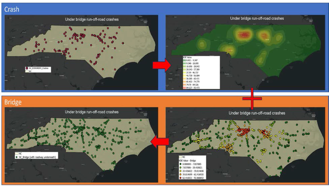
To estimate the spatial distribution of BrTSs, kernel density estimation (KDE) of crash data is recommended. One advantage of utilizing KDE is that the method does not require the linkage between crashes and specific bridges. KDE creates heatmap using all geocoded crashes, making it easy to see where crash hot spots are located on a large scale. KDE values can then be assigned to individual bridges by superimposing the bridge layer over the BrTS heatmap. This way, the risk score can be determined based on the KDE values. Figure 12 shows an example of the crash heatmap for under-bridge strikes (with substructure) in North Carolina.
Expert Knowledge
The expert knowledge risk assessment relies on individuals who have extensive knowledge and experience in a particular field to evaluate risks. In the context of bridge safety, experts with relevant knowledge and experience are typically engineers or other professionals who specialize in transportation or bridge engineering.
This method involves a systematic evaluation of various risk factors. Experts use their professional judgement and expertise to evaluate each risk factor and assign a score to each one based on the level of risk it poses to bridge safety. The score assigned to each risk factor may also be based on previous research and industry standards. After the scores for each risk factor have been assigned, risk factors are combined to produce an overall risk score for each bridge. The overall risk score is used to prioritize bridges for further inspection, repair or maintenance. One of the benefits of this method is its flexibility and how easy it is to customize data depending on local knowledge and data availability. Therefore, this method is particularly useful in situations where data may be limited or incomplete.
NYSDOT’s CVA is an example of an expert knowledge-based risk assessment method. CVA has been used for many decades to determine the relative vulnerability of the state’s bridges to failures caused by impact damages (Agrawal, Xu, and Chen 2011). A collision vulnerability rating is calculated for each
bridge using the CVA procedure, which involves a series of assessment and evaluation steps tailored to the bridge’s unique features. This rating indicates the probability and consequences of failures, specifying the necessary corrective actions to mitigate vulnerability and the urgency of their implementation.
However, one of the drawbacks of this method is that it may be subjective and may not be reproducible across other experts. Additionally, the selection and weights of risk factors are not necessarily determined by data and rigorous statistical models, but by experts’ opinions. Therefore, it is important to ensure that the experts conducting the assessment have a strong understanding of the risk factors and that there is consistency in the approach used by each expert. Nevertheless, the expert knowledge-based risk assessment can be a valuable tool for evaluating bridge safety and prioritizing maintenance and inspection efforts, especially when data are not available, or reliable.
Crash Prediction Model
Another viable option for prioritizing locations for safety improvement measures is to use a statistical model to predict the probability of crash occurrences. With this approach, an agency can assign a risk score to each location based on the model prediction. The statistical model assigns a weight to each factor that affects the likelihood of a crash. The coefficients estimated during the modeling process serve as the weights for each risk factor, thereby eliminating the use of subjective weights.
The industry standard for predictive crash modeling is a negative binomial (NB) crash count model. This statistical model allows agencies to estimate the number of BrTSs that may occur at a particular location, based on site-specific characteristics such as roadway geometry, traffic volume, and historical crash data. The NB model accounts for the overdispersion often observed in crash data (where the variance is greater than the mean) by incorporating a dispersion parameter in the model. Additionally, the model can be calibrated to reflect the specific context of the agency, such as a certain type of BrTS crashes or the specific characteristics of the study area. The following equation is a general functional form for a statistical model applied in this project to predict BrTS crashes:
Where:
– BrTS Crashesi is the estimated bridge strikes at bridge i
– Structure Length is the length of the structure defined as:
– Length of bridge structure for on-bridge strikes (e.g., truss, parapet, railing)
– Length of deck for both under-bridge strikes with overhead structure (e.g., girder) and under-bridge strikes with pier or support (e.g., bent, support, pier, abutment)
– n is the number of years considered for the study (i.e., 5 years)
– AADT is the annual average daily traffic (based on the type of the estimated crash)
– xij is the quantitative measure of each explanatory variable j associated with bridge i
– α and βj are estimated model coefficients for the explanatory variable j
– β0 is the estimated constant.
In addition to the crash count model, an outcome model that calculates the monetized value of the comprehensive costs of a crash could also be considered. The outcome model can be established for both loss of life and structural damage based on the availability of data. The following equation is an example of the most popular multinomial logit (MNL) model for outcome modeling:
Where:
– Pij is the probability of ith vehicle-bridge strike with jth personal injury severity level outcome
– Xij denotes the vector of observable factors (variables) for ith vehicle-bridge strike with jth injury severity level
– αj is the estimated constant
– βj represents the vector of estimated coefficients.
Considering the practicality of the methodology from a broad perspective, only personal injury severity is considered instead of failure of structure (e.g., catastrophic collapse, partial collapse, structure damage, or actual damage costs in money value) to represent the impact of BrTS.
Thus, the impacts resulting from both aspects can be quantified through a two-step approach combining both crash count model and the outcome model. The effects of significant risk factors in the developed models can be retrieved to help evaluate the BrTS risk for structures and identify proper treatments. It is also possible to combine the results from the modeling with the cost-benefit analysis for different treatments. The entire concept is demonstrated in Figure 13.
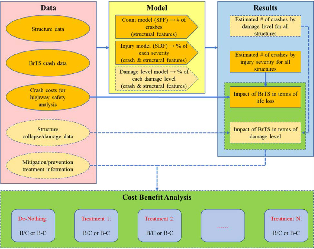
A complete development of such a modeling work using sample data by the project team can be found in Appendix D: Technical Memorandum: Crash Prediction Models for Highway Bridges, which includes comprehensive procedures, results, and their interpretations.
Case Studies
In addition to the general frameworks of the risk assessment methods described early in this chapter, the project team has also identified several case studies from the existing research and by state agencies projects built upon the literature review. The intent was to analyze, summarize, and document the practical methods and tools that state agencies developed and used. This includes six case studies performed by the NYSDOT, Alabama DOT (ALDOT), Florida DOT (FDOT), Iowa DOT, South Dakota DOT (SDDOT), and Texas DOT (TxDOT), respectively. All except for the NYSDOT are focused on a particular type of bridge collision. The detailed summary can be found in Appendix E: Technical Memorandum: Case Studies.


