Data collected in the departmental and faculty surveys were used to answer various research questions in this report. Statistical analyses consisted essentially of fitting various types of regression models, including multiple linear regression, logistic regression, and Poisson regression models depending on the distributional assumptions that were appropriate for each response variable of interest. In some cases, the response variable was transformed so that the assumption of normality for the response in the transformed scale was plausible. Marginal or least-squares means were calculated (sometimes in the transformed scale) for effects of interest in the models.

We let y denote a response variable such as the proportion of women in the applicant pool or annual salary or number of manuscripts published in a year, and use x to denote a vector of covariates that might include type of institution, discipline, proportion of women on the search committee, etc. If y can be assumed to be normally distributed with some mean μ and some variance σ² then we typically fit a linear regression model to y that establishes that μ = xβ, where β is a vector of unknown regression coefficients.

When the response y is not normally distributed (for example, because y can only take on values 0 and 1) then we can define η = xβ and then choose a transformation g of μ such that

For example, if the response variable is a proportion, the logit transformation

is appropriate. When y is a count variable (as in the number of manuscripts published in a year) the usual transformation is the log transformation.

One approach to obtaining estimates of β is the method of maximum likelihood. Let denote the maximum likelihood estimate (MLE) of β. A nice property of MLEs is invariance; in general, the MLE of a function h(β) is equal to the function of the MLE of β, thus

In particular, if then

The difficulty arises when we wish to also estimate the variance of for example to then obtain a confidence interval around the point estimate . To do so, we typically need to resort to linearization techniques that allow us to compute an approximation to the variance of a non-linear function of the parameters. A method that can be used for this purpose is called the Delta method and is described below.

Least-squares means of the response, also known as adjusted means or marginal means can be computed for each classification or qualitative effect in the model. Examples of qualitative effects in our models include type of institution (two levels: public or private) discipline (with six categories in our study), gender of chair of search committee, and others. Least-squares means are predicted population margins or within-effect level means adjusted for the other effects in the model. If the design is balanced, the least-squares means (LSM) equal the observed marginal means. Our study design is highly unbalanced and thus the LSM of the response variable for any effect level will not coincide with the simple within-effect level mean response.

Each least-squares mean is computed as for a given vector L. For example, in a model with two factors A and B, where A has three levels and B has two levels, the least squares mean response for the first level of factor A is given by:

where the first coefficient 1 in L corresponds to the intercept, the next three coefficients correspond to the three levels of factor A and the last two coefficients correspond to the two levels of factor B. If the model also includes an interaction between A and B, then L and has an additional 3 × 2 elements. The corresponding values of the additional six elements in L would be ½ for the two interaction levels involving the first level of factor A (A₁B₁, A₁B₂ ) and 0 for the four interaction levels that do not involve the first level of factor A (A₂B₁, A_sB₂, A₃B₁, A₃B₂). The coefficient vector L is constructed in a similar way to compute the LSM of y (or a transformation of y) for the remaining two levels of A, two levels of B, and even for the six levels of the interaction between A and B if it is present in the model.

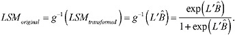
When the response variable has been transformed prior to fitting the model, the LSM is computed in the transformed scale and must be then transformed back into the original scale. If we have MLEs of the regression coefficients, we can easily compute the LSMs in the original scale simply by applying the inverse

transformation to . For example, if g(μ) = log(μ) = xβ and is the least squares mean in the transformed scale, we can compute the LSM in the original scale as

If the transformation was the logit transformation, the LSM in the original scale is computed as

Suppose that we fit a model to a response variable that has been transformed using some function g as above, and obtain an estimate of a mean . Programs including SAS will also output an estimate of the variance of . We can compute the estimate of the mean in the original scale by applying the inverse transformation g^–1 to as described above. In order to obtain an estimate of the variance of , however, we need to make use of, for example, the Delta method, which we now explain.

Given any non-linear function H of some scalar-valued random variable θ, H(θ) and given σ², the variance of θ, we can obtain an expression for the variance of H(θ) as follows:

For example, suppose that we used a log transformation on a response variable and obtained an LSM in the transformed scale that we denote , with estimated variance . The estimate of the mean in the original scale is obtained by applying the inverse transformation to the LSM:

The variance of is given by:

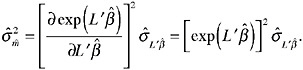
Suppose now that the response variable was binary and that we used a logit transformation so that

Given an MLE and an estimate of the least squares mean in the transformed scale, we compute and as follows:

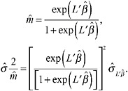
Given a point estimate of the least squares mean in the original scale and an approximation to its variance, we can compute an approximate 100(1–α)% confidence interval for the true mean in the original scale in the usual manner:

where df is the appropriate degrees of freedom. In our case, and due to relatively large sample sizes everywhere, the t critical value can be replaced by the corresponding upper α/2 tail of the standard normal distribution.