Reference Manual on Scientific Evidence: Fourth Edition (2025)
Chapter: Reference Guide on Statistics and Research Methods
Reference Guide on Statistics and Research Methods
DAVID H. KAYE AND HAL S. STERN
David H. Kaye, M.A., J.D., is Regents Professor Emeritus, Arizona State University Sandra Day O’Connor College of Law and School of Life Sciences, and Distinguished Professor of Law and Academy Professor Emeritus, Pennsylvania State University School of Law.
Hal S. Stern, Ph.D., is Distinguished Professor, Department of Statistics, University of California, Irvine.
Authors’ Note: Research for this reference guide was completed in 2023. Professor David A. Freedman co-authored the first three editions of this reference guide. His writing and thinking are evident throughout this edition as well.
CONTENTS
Admissibility and Weight of Statistical Studies
Varieties and Limits of Statistical Expertise
Procedures That Enhance Statistical Testimony
Maintaining Professional Autonomy
Disclosing Limitations and Other Analyses
Disclosing Data and Analytical Methods Before Trial
How Have the Data Been Collected?
Is the Study Designed to Investigate Causation?
Randomized Controlled Experiments
Descriptive Surveys and Censuses
What Method Is Used to Select the Units?
Of the Units Selected, Which Provide Measurements?
Is the Measurement Process Reliable?
Is the Measurement Process Valid?
How Have the Data Been Presented?
Are Rates or Percentages Properly Interpreted?
How Big Is the Base of a Percentage?
Have Appropriate Benchmarks Been Provided?
Have the Data Collection Procedures Changed?
Are the Categories Appropriate?
Is an Appropriate Measure of Association Used?
Does a Graph Portray Data Fairly?
How Are Distributions Displayed?
Is an Appropriate Measure Used for the Center of a Distribution?
Is an Appropriate Measure of Variability Used?
What Inferences Can Be Drawn from the Data?
What Estimator Should Be Used?
What Is the Confidence Interval?
The normal curve and large samples
What Are the Technical and Interpretive Difficulties with Confidence Intervals?
p-values, Significance Levels, and Hypothesis Tests
Is a Difference Statistically Significant?
Recent Emphasis on the Limitations of p-values
Is the Sample Statistically Significant?
What Is the Power of the Test?
How Many Tests Have Been Done?
What Are the Rival Hypotheses?
Bayesian Statistical Methods and Posterior Probabilities
Do Outliers Influence the Correlation Coefficient?
Does a Confounding Variable Influence the Coefficient?
Data Science and Statistical Machine Learning
What Statistical Questions Arise with Machine Learning Studies?
Is the Dataset Appropriate and of Sufficient Quality?
Is the Predictor or Classifier Robust?
Is the Predictor or Classifier Too Opaque?
Appendix: Conditional Probability and Bayes’ Rule
What Do Probabilities Apply To?
What Are Conditional Probabilities?
References on Statistics and Research Methods
FIGURES
1 and 2. Manipulating the scale of a graph
5. Plotting points in a scatter diagram
6. Scatter diagram for income and education: men ages 25 to 34 in Kansas
7. The correlation coefficient measures the sign of a linear association, and its strength
8. A strong nonlinear association with a correlation coefficient close to zero
9. The correlation coefficient can be distorted by outliers
10. The regression line for income on education and its estimates
11. Scatter diagram for income and education, with the regression line indicating the trend
TABLES
1. Test Results for Cartridge-case Comparisons
2. Data Used by a Defendant to Refute Plaintiff’s False Advertising Claims
3. Home Pregnancy Test Results
Introduction
Statistical assessments are prominent in many kinds of legal cases, including antitrust, employment discrimination, toxic torts, and voting rights cases. This reference guide describes the elements of statistical reasoning. We hope the explanations will help judges and lawyers to understand statistical terminology, to see the strengths and weaknesses of statistical arguments, and to apply relevant legal doctrine. The guide is organized as follows:
- This introduction provides an overview of the field, discusses the admissibility of statistical studies, and offers some suggestions about procedures that encourage the best use of statistical evidence.
- The section titled “How Have the Data Been Collected?” addresses data collection. It explains why the design of a study is the most important determinant of its quality. The section compares experiments with observational studies and surveys with censuses, indicating when the various kinds of study are likely to provide useful results.
- The section titled “How Have the Data Been Presented?” discusses the art of summarizing data. This section considers the mean, median, and standard deviation. These are basic descriptive statistics, and most statistical analyses use them as building blocks. This section also discusses patterns in data that are brought out by graphs, percentages, and tables.
- The section titled “What Inferences Can Be Drawn from the Data?” describes the logic of statistical inference, emphasizing foundations and disclosing limitations. This section covers estimation, standard errors and confidence intervals, p-values, and hypothesis tests.
- The section titled “Correlation and Regression” shows how associations can be described by scatter diagrams, correlation coefficients, and regression lines. Regression is often used in attempts to infer causation from association. This section explains the technique, indicating the circumstances under which it and other statistical models are likely to succeed—or fail.
- Advances in computing speed and the availability of large datasets have made it possible to fit models of greater complexity than those described in the section titled “Correlation and Regression.” The section titled “Data Science and Statistical Machine Learning” describes the developing fields of “data science” and “machine learning” and statistical issues that affect the confidence one can have in the output of machine-learning techniques.
- An appendix discusses the scope of the theory of probability, conditional probabilities, Bayes’ rule, and perspectives on statistical inference.
- The glossary defines statistical terms that may be encountered in litigation, including ones that do not appear in the body of the guide.
Admissibility and Weight of Statistical Studies
Statistical studies suitably designed to address a material issue generally will be admissible under the Federal Rules of Evidence. The hearsay rule rarely is a serious barrier to the presentation of statistical studies, because such studies may be offered to explain the basis for an expert’s opinion or may be admissible under the learned treatise exception to the hearsay rule.1 Most statistical methods applied in litigation are described in textbooks or journal articles and are capable of producing useful results when properly applied. As such, these methods generally satisfy important aspects of the “scientific knowledge” requirement in Daubert v. Merrell Dow Pharmaceuticals, Inc.2 However, a particular study may use a method that is entirely appropriate but so poorly executed that it should be inadmissible under Federal Rules of Evidence 403 and 702.3 Or, the method may be inappropriate for the problem at hand and thus lack the “fit” referred to in Daubert.4 Or the study might rest on data of the type not reasonably relied on by statisticians or substantive experts and hence not be suitable as a basis for an opinion under Rule 703. Often, however, the battle over statistical evidence concerns weight or sufficiency rather than admissibility.
Varieties and Limits of Statistical Expertise
For convenience, the field of statistics may be divided into three subfields: probability theory, theoretical statistics, and applied statistics. Probability theory is the mathematical study of outcomes that are governed, at least in part, by chance. Theoretical statistics is about understanding the properties of statistical procedures, including error rates; probability theory plays a key role in this endeavor. Applied statistics draws on both these fields to develop techniques for collecting or analyzing particular types of data.
Statistical expertise is not confined to witnesses with degrees in statistics. Because statistical reasoning underlies many kinds of empirical research, scholars in a variety of fields—including biology, business, economics, epidemiology, medicine, political science, psychology, and sociology—are exposed to statistical ideas, with an emphasis on the methods most important to the discipline. The diffusion of statistical concepts and methods across so many fields raises the question
1. See generally 2 McCormick on Evidence §§ 321, 324.3 (Robert P. Mosteller ed., 8th ed. 2020). Studies published by government agencies also may be admissible as public records. Id. § 296.
2. 509 U.S. 579, 589–90 (1993).
3. See Kumho Tire Co. v. Carmichael, 526 U.S. 137, 152 (1999) (suggesting that the trial court should “make certain that an expert, whether basing testimony upon professional studies or personal experience, employs in the courtroom the same level of intellectual rigor that characterizes the practice of an expert in the relevant field”).
4. Daubert, 509 U.S. at 591.
of who is qualified to conduct and testify to statistical assessments—a statistical methodologist, a substantive scientist, or both? Much depends on context.
If the study involves assembling and then analyzing case-specific data, the choice of which data to examine and how best to model a particular process could require both subject-matter and general statistical expertise. The two types of expertise might be combined in a single individual. A labor economist, for example, should be able to supply a definition of the relevant labor market from which an employer draws its employees. This economist also might be sufficiently educated in statistical tests for group differences to compare the race of new hires to the racial composition of the labor market. When the analysis is as straightforward as the comparison of two proportions, a single substantive expert may suffice.5 But further analysis of the possible reasons for the racial disparity might require input from an expert with an understanding of more advanced methods. This expert might be a statistician or an econometrician, or a scientist or engineer who works with other data in a completely different field of study.
The critical question is whether the individual has the education and experience to determine which statistical techniques are appropriate for the task at hand and to apply such techniques with an appreciation of their limitations. Experts who specialize in using statistical methods, and whose professional careers demonstrate this orientation, are most likely to use appropriate procedures and correctly interpret the results. To ascertain the extent to which an expert has this orientation and acumen, one can look to formal education, professional accomplishments, and reputation in the pertinent community of experts. Has the individual studied quantitative methods? Taught them? Used them in research? Which ones? If the expert is or was an academic professional, a university teaching portfolio with courses on statistical methods is a good sign. Ideally, the publication and research record will include studies that use or describe the same or similar methods as those applied (or applicable) to the case at bar.6 Invitations from mainstream journal editors to review articles submitted for publication, from academic conference organizers to present research involving statistics, and from government regulatory and research agencies to serve on expert panels that evaluate statistical work are further indications of recognized expertise within a statistical discipline. General membership in most scientific and professional societies requires no special accomplishments, but certain designations, prizes, or awards from such organizations for scholarship are a sign that an
5. Of course, the case could be presented in the form of interlocking testimony from two experts—the labor economist followed by any expert with the appropriate expertise in the method for making the statistical comparison. The substantive knowledge may be of lesser value in selecting a statistical model. Various models might be consistent with the substantive knowledge, and there may be purely statistical criteria for choosing among them.
6. Academic experts are likely to have a long list of publications, but length alone is not the best indication of pertinent expertise. Not all publishers are equal, and every field has a relatively small number of top-tier journals.
expert’s work has had an impact. Of course, these factors are merely indicia of degrees of expertise and specialization. Highly competent work can be done by individuals with shorter curricula vitae.
Again, not every case involving computations of probability or statistics necessitates a highly skilled statistical specialist. Medical practitioners and forensic scientists who are not statistical specialists often make statistical assessments of evidence or rely on and present the results of statistical studies. In these situations, it is important to ensure that the witnesses do not exceed the bounds of their statistical expertise. The scientist or practitioner might lack basic information about the studies underlying their testimony. State v. Garrison7 illustrates the problem. In this murder prosecution involving bitemark evidence, a dentist was allowed to testify that “the probability factor of two sets of teeth being identical in a case similar to this is, approximately, eight in one million,” even though “he was unaware of the formula utilized to arrive at that figure other than that it was ‘computerized.’”8 Likewise, laboratory analysts or examiners may have only a limited understanding of the foundations of automated systems for comparing patterns within DNA samples, toolmarks, fingerprints, voice recordings, and the like. Once the formulas or methods have been shown to work well, and when their limitations and proper use are known, the practitioners may be qualified to operate the statistical machinery, as it were, without an in-depth understanding of the routinized or automated statistical or probabilistic method. But the operational training may not qualify them to explain the developmental research. They may have to limit their statistical testimony to an explanation of how they arrived at their estimates and to statements of the extent to which software or hardware is used in practice and whether there are publications on its validity.
Procedures That Enhance Statistical Testimony
Maintaining Professional Autonomy
Ideally, experts who conduct research in the context of litigation should proceed with the same objectivity that would be required in other professional contexts. Thus, experts who testify (or who supply results used in testimony) should conduct the analysis required to address, in a professionally responsible fashion, the issues posed by the litigation.9 Questions about the freedom of inquiry accorded
7. 585 P.2d 563 (Ariz. 1978).
8. Id. at 566, 568. For other examples, see David H. Kaye et al., The New Wigmore: A Treatise on Evidence: Expert Evidence § 12.2 (2d ed. 2011).
9. See Nat’l Research Council Panel, The Evolving Role of Statistical Assessments as Evidence in the Courts 164 (Stephen E. Fienberg ed., 1989) [hereinafter NRC Panel] (recommending that the expert be free to consult with colleagues who have not been retained by any party to the litigation and that the expert receive a letter of engagement providing for these and other safeguards).
to testifying experts, as well as the scope and depth of their investigations, may reveal some of the limitations to the testimony.
Disclosing Limitations and Other Analyses
Statisticians analyze data using a variety of methods. To permit a fair evaluation of the analysis that is eventually settled on, the testifying expert can be asked how that approach was developed, whether alternative approaches were considered, and, if so, what the results were.10 Ethical guidelines for statisticians require them to disclose known and suspected limitations in the data and its analysis.11
Disclosing Data and Analytical Methods Before Trial
The collection of data often is expensive and subject to errors and omissions. Moreover, careful exploration of the data can be time-consuming. To minimize debates at trial over the accuracy of data and the choice of analytical techniques, pretrial-discovery procedures should be used, particularly with respect to the quality of the data and the method of analysis.12 In some cases, these could include requirements for specifying in detail the study design and analysis that are planned before data collection begins.13
10. Id. at 167; cf. Edith Beerdsen, Litigation Science After the Knowledge Crisis, 106 Cornell L. Rev. 529 (2021) (discussing responses to the “replication crisis” in the academic biomedical and behavioral science publication process and suggesting pretrial procedures to make the exercise of “analytical flexibility” in “litigation science” more transparent); Yoav Benjamini, Selective Inference: The Silent Killer of Replicability, 2 Harv. Data Sci. Rev. (2020), https://doi.org/10.1162/99608f92.fc62b261 (noting the problem of presenting or emphasizing selected findings within scientific publications).
11. ASA Comm. on Professional Ethics, Ethical Guidelines for Statistical Practice, Feb. 2022, at 3 & 4, https://perma.cc/P4P6-JU6C. Invoking an attorney’s professional duty not to intentionally mislead the courts on the facts or the law, the Panel on Statistical Assessments as Evidence insisted that “it is not appropriate for the attorney to seek to avoid such revelation [of alternative forms of data and analyses] by consulting a series of experts without revealing to the experts ultimately retained any prior history of the involvement of other experts in the litigation.” NRC Panel, supra note 9, at 167.
12. See The Special Comm. on Empirical Data in Legal Decision Making, Recommendations on Pretrial Proceedings in Cases with Voluminous Data, reprinted in NRC Panel, supra note 9, app. F; David H. Kaye, Improving Legal Statistics, 24 Law & Soc’y Rev. 1255 (1990).
13. Drawing on “open science” practices, commentators have proposed adaptations of practices for “registration” of academic research studies. See Beerdsen, supra note 10; section titled “Recent Emphasis on the Limitations of p-values” below.
How Have the Data Been Collected?
The interpretation of data often depends on understanding “study design”—the plan for a statistical study and its implementation.14 Different designs are suited to answering different questions. Also, flaws in the data can undermine any statistical analysis, and data quality is often determined by study design.
In many cases, statistical studies are used to show causation. Do food additives cause cancer? Does capital punishment deter crime? Would additional disclosures in a securities prospectus cause investors to behave differently? The design of studies to investigate causation is the first topic of this section.15
Sample data can be used to describe a population. The population is the whole class of units that are of interest; the sample is the set of units chosen for detailed study. Inferences from the part to the whole are justified when the sample is representative. Sampling is the second topic of this section.
Finally, issues associated with the reliability and accuracy of collected data will be considered. Measurement error should be assessed and the likely impact of errors considered. Data quality is the third topic of this section.
All the sections concern the study of “variables.” In statistics, a variable is a characteristic of the units in a study. With a study of people, the unit of analysis is the person, and the variables describe people. Two such variables would be income (dollars per year) and educational level (years of schooling completed). With a study of school districts, the unit of analysis is the district. Typical variables include average family income of district residents and average test scores of students in the district.
Variables may be related to one another in various ways. Many studies examine whether a variable or group of variables, known as independent variables, are related to an outcome or dependent variable. For example, census data can be analyzed to determine whether people who complete more years of school tend to have higher incomes later in life. Educational level would be the independent variable, and annual income the dependent variable. In a study of smoking and lung cancer, the independent variable could be smoking (perhaps measured by the number of cigarettes smoked per day), and the dependent variable could mark the presence or absence of lung cancer.
14. For introductory treatments of data collection, see, for example, David Freedman et al., Statistics (4th ed. 2007); Darrell Huff, How to Lie with Statistics (1993); David S. Moore & William I. Notz, Statistics: Concepts and Controversies (10th ed. 2019); Hans Zeisel, Say It with Figures (6th ed. 1985); Hans Zeisel & David Kaye, Prove It with Figures: Empirical Methods in Law and Litigation (1997).
15. See also Steve C. Gold et al., Reference Guide on Epidemiology, “The Different Kinds of Epidemiologic Studies” section, in this manual.
Is the Study Designed to Investigate Causation?
Types of Studies
When causation is the issue, anecdotal evidence can be brought to bear. So can observational studies or controlled experiments. Anecdotal reports may be of value, but they are ordinarily more helpful in generating lines of inquiry than in proving causation. In medicine, evidence from clinical practice can be a good starting point for discovery of cause-and-effect relationships, but the anecdotal experience of practitioners is not definitive.16 Observational studies can establish that one factor is associated with another, but work is needed to bridge the gap between association and causation. Randomized controlled experiments are ideally suited for demonstrating causation.
Anecdotal evidence usually amounts to reports that events of one kind are followed by events of another kind. Typically, the reports are not even sufficient to show association, because there is no comparison group. For example, some children who live near power lines develop leukemia. Does exposure to electrical and magnetic fields cause this disease? The anecdotal evidence is not compelling because leukemia also occurs among children without exposure.17 It is necessary to compare disease rates among those who are exposed and those who are not. If exposure causes the disease, the rate should be higher among the exposed and lower among the unexposed. That would be association.
16. Consequently, many courts have suggested that attempts to infer causation from anecdotal reports are inadmissible as unsound methodology under Daubert v. Merrell Dow Pharmaceuticals, Inc., 509 U.S. 579 (1993). See, e.g., Miller v. Pfizer, Inc., 356 F.3d 1326, 1331 (10th Cir. 2004) (affirming the district court’s exclusion in part because “placing substantial emphasis on a few challenge-dechallenge-rechallenge studies and case reports is not a generally accepted methodology”); Hendrix ex rel. G.P. v. Evenflo Co., Inc., 609 F.3d 1183 (11th Cir. 2010) (“Case studies and clinical experience, used alone and not merely to bolster other evidence, are . . . insufficient to show general causation.”); cf. Matrixx Initiatives, Inc. v. Siracusano, 563 U.S. 27, 44 (2011) (concluding that adverse-event reports combined with other information could be of concern to a reasonable investor and therefore subject to a requirement of disclosure under SEC Rule 10b-5, but stating that “the mere existence of reports of adverse events . . . says nothing in and of itself about whether the drug is causing the adverse events”). Other courts are more open to “differential diagnoses” based primarily on timing. E.g., Best v. Lowe’s Home Ctrs., Inc., 563 F.3d 171 (6th Cir. 2009) (reversing the exclusion of a physician’s opinion that exposure to propenyl chloride caused a man to lose his sense of smell because of the timing in this one case and the physician’s inability to attribute the change to anything else).
17. See Nat’l Research Council, Possible Health Effects of Exposure to Residential Electric and Magnetic Fields (1997). There are problems in measuring exposure to electromagnetic fields, and results are inconsistent from one study to another. For such reasons, the epidemiologic evidence for an effect on health is inconclusive. Nat’l Cancer Inst., Electromagnetic Fields and Cancer, May 30, 2022 (“Studies have examined associations of these cancers with living near power lines, with magnetic fields in the home, and with exposure of parents to high levels of magnetic fields in the workplace. No consistent evidence for an association between any source of non-ionizing EMF and cancer has been found.”).
The next issue is crucial: Exposed and unexposed people may differ in ways other than the exposure they have experienced. For example, children who live near power lines could come from poorer families and be more at risk from other environmental hazards. Such differences can create the appearance of a cause- and-effect relationship. Other differences can mask a real relationship. Cause-and-effect relationships often are quite subtle, and carefully designed studies are needed to draw valid conclusions.
An epidemiological classic makes the point. At one time, it was thought that lung cancer was caused by fumes from tarring the roads, because many lung cancer patients lived near roads that recently had been tarred. This is anecdotal evidence. But the argument is incomplete. For one thing, most people—whether exposed to asphalt fumes or unexposed—did not develop lung cancer. A comparison of rates was needed. Epidemiologists found that exposed persons and unexposed persons suffered from lung cancer at similar rates: Tar was probably not the causal agent. Exposure to cigarette smoke, however, turned out to be strongly associated with lung cancer. This study, in combination with later ones, made a compelling case that smoking cigarettes is the main cause of lung cancer.18
A good study design compares outcomes for subjects who are exposed to some factor (the treatment group) with outcomes for other subjects who are not exposed (the control group). With comparison groups, there is another important distinction—between controlled experiments and observational studies. In a controlled experiment, the investigators decide which subjects will be exposed and which subjects will be in the control group. In observational studies, the researchers do not determine which subjects are exposed; often, the subjects themselves choose their exposures. Because of self-selection or for other reasons, the treatment and control groups are likely to differ with respect to influential factors other than the ones of primary interest. These other factors are called lurking variables or confounding variables.19 A confounding variable can be correlated with the independent variable and act causally on the dependent variable. When
18. Richard Doll & A. Bradford Hill, A Study of the Aetiology of Carcinoma of the Lung, 2 Brit. Med. J. 1271 (1952), https://doi.org/10.1136/bmj.2.4797.1271. This was a matched case-control study. Cohort studies soon followed. See Gold et al., supra note 15. For a review of the evidence on causation, see 38 Int’l Agency for Research on Cancer (IARC), World Health Org., IARC Monographs on the Evaluation of the Carcinogenic Risk of Chemicals to Humans: Tobacco Smoking (1986) (updated 100E, A Review of Human Carcinogens: Personal Habits and Indoor Combustions 43–211 (2012)).
19. Epidemiologists sometimes limit “confounding” to “a bias due to the existence of a common cause of exposure and outcome” and define “selection bias” as “bias by [selecting units for study based] on common effects of otherwise unrelated variables.” Stephen R. Cole et al., Illustrating Bias Due to Conditioning on a Collider, 39 Int’l J. Epidemiology 417, 420 (2010), https://doi.org/10.1093/ije/dyp334. The distinction can be helpful in spotting different threats to causal inference, but this section uses the terms more loosely.
that happens, the confounder—not the independent variable—could be responsible for differences seen on the dependent variable. With the health effects of power lines, family background is a possible confounder; so is exposure to other hazards. Many confounders have been proposed to explain the association between smoking and lung cancer, but careful epidemiological studies have ruled them out, one after the other.
Confounding remains a problem even for the best observational research. For example, women with herpes are more likely to develop cervical cancer than other women. Some investigators concluded that herpes caused cancer: In other words, they thought the association was causal. Later research showed that the primary cause of cervical cancer was human papilloma virus (HPV). Herpes was a marker of sexual activity. Women who had multiple sexual partners were more likely to be exposed not only to herpes but also to HPV. The association between herpes and cervical cancer was due to other variables.20
Randomized Controlled Experiments
In randomized controlled experiments, investigators assign subjects to treatment or control groups at random. The groups are therefore likely to be comparable, except for the treatment. This minimizes the role of confounding. Minor imbalances will remain, owing to the play of random chance; the likely effect on study results can be assessed by statistical techniques.21 The bottom line is that causal inferences based on well-executed randomized experiments are generally more secure than inferences based on well-executed observational studies.
The following example should help bring the discussion together. Today, we know that taking aspirin helps prevent heart attacks. But initially, there was some controversy. People who take aspirin rarely have heart attacks. This is anecdotal evidence for a protective effect, but it proves almost nothing. After all, few people have frequent heart attacks, whether or not they take aspirin regularly. A good study compares heart-attack rates for two groups: people who take aspirin (the treatment group) and people who do not (the controls). An observational study would be easy to do, but in such a study the aspirin-takers are likely to be different from the controls. Indeed, they are likely to be sicker—that is why they are taking aspirin. The study would be biased against finding a protective effect.
20. For additional examples and further discussion, see David A. Freedman, From Association to Causation: Some Remarks on the History of Statistics, 14 Stat. Sci. 243 (1999). Some studies find that herpes is a “cofactor,” which increases risk among women who are also exposed to HPV. Only certain strains of HPV are carcinogenic.
21. Randomization of subjects to treatment or control groups puts statistical tests of significance on a secure footing. See section titled “What Inferences Can Be Drawn from the Data?” below.
Randomized experiments are harder to do, but they provide better evidence.22 The experiments demonstrate the protective effect.23
In summary, data from a treatment group without a control group generally reveal very little and can be misleading. Comparisons are essential. If subjects are assigned to treatment and control groups at random, a difference in the outcomes between the two groups can usually be accepted, within the limits of statistical error,24 as a good measure of the treatment effect. However, if the groups are created in any other way, differences that existed before treatment may contribute to differences in the outcomes or mask differences that otherwise would become manifest. Observational studies succeed to the extent that the treatment and control groups are comparable—apart from the treatment.
Observational Studies
The bulk of the statistical studies seen in court are observational, not experimental. Take the question of whether capital punishment deters murder. To conduct a randomized controlled experiment, people would need to be assigned randomly to a treatment group or a control group. People in the treatment group would know they were subject to the death penalty for murder; the controls would know that they were exempt. Conducting such an experiment is not possible.
Many studies of the deterrent effect of the death penalty have been conducted, all observational, and some have attracted judicial attention. Researchers have catalogued differences in the incidence of murder in states with and without the death penalty and have analyzed changes in homicide rates and execution rates over the years. When reporting on such observational studies, investigators may speak of “control groups” (e.g., the states without capital punishment) or claim they are “controlling for” confounding variables by statistical methods such as multiple regression.25 However, association is not causation. The
22. One important feature of a clinical trial is “blinding” to prevent unconscious bias. In a “double blind” trial, neither the patients nor the clinicians ascertaining the outcomes know who received the treatment and who did not. This prevents the expectations of the subjects and the experimenters from systematically affecting the observed outcomes in one group relative to the other.
23. But randomized experiments also show that aspirin can cause internal bleeding, raising the practical questions of whether and when a low-dose regimen is more beneficial than harmful. See, e.g., U.S. Preventive Services Task Force, Aspirin Use to Prevent Cardiovascular Disease: Preventive Medication, Apr. 26, 2022, https://perma.cc/C8V9-WMYS. In other instances, experiments have contradicted strongly held beliefs. E.g., Eric A. Klein et al., Vitamin E and the Risk of Prostate Cancer: Results of the Selenium and Vitamin E Cancer Prevention Trial (SELECT), 306 JAMA 1549 (2011), https://doi.org/10.1001/jama.2011.1437.
24. See section titled “What Inferences Can Be Drawn from the Data?” below.
25. Multiple regression is described in Daniel L. Rubinfeld & David Card, Reference Guide on Multiple Regression and Advanced Statistical Models, in this manual. On the limits of regression to cope
causal inferences that can be drawn from analysis of observational data—no matter how complex the statistical technique—usually rest on a foundation that is less secure than that provided by randomized controlled experiments.
When an external change in circumstances naturally creates a treatment and a control group in a manner that is comparable to random assignment by the researchers, the study may be called a “natural experiment” or a “quasi-experiment.”26 A celebrated example comes from Dr. John Snow’s investigation of cholera and sewage in the mid-1800s. The residents of an area in London received water from two companies with overlapping water mains drawing from a part of the Thames River that was heavily polluted with raw sewage. Then, one company moved its water intake upstream, to a less polluted spot. Snow showed that during a London cholera epidemic soon afterwards, the death rates from cholera in homes with the less polluted water was less than one-eighth that for the more polluted homes—and less than that for the rest of London.27 Snow argued that “no experiment could have been devised which would more thoroughly test the effect of water supply on the progress of cholera than this . . . .”28 In modern terminology, the argument is that even though the study was observational, the seemingly random assignment of homes to the two intake points protects against confounding and bias.
Observational studies can be very useful even when assignments to the groups being compared do not resemble randomization imposed by an experimenter. For example, there is strong observational evidence that smoking causes lung cancer (see section titled “Types of Studies” above). Generally, observational studies provide good evidence in the following circumstances:
- The association is seen in studies with different designs, on different kinds of subjects, and done by different research groups.29 That reduces the chance that the association is due to a defect in one type of study, a peculiarity in one group of subjects, or the idiosyncrasies of one research group.
with lurking variables, see Richard A. Berk, Regression Analysis: A Constructive Critique (2004); Richard Berk, What You Can and Can’t Properly Do with Regression, 26 J. Quantitative Criminology 481 (2010), https://doi.org/10.1007/s10940-010-9116-4; David A. Freedman, Statistical Models: Theory and Practice (2005).
26. See, e.g., Frank de Vocht et al., Conceptualising Natural and Quasi Experiments in Public Health, 21 BMC Med. Research Methodology 32 (2021), https://doi.org/10.1186/s12874-021-01224-x.
27. John Snow, On the Mode of Transmission of Cholera 55–98 (2d ed. 1855).
28. Id. at 46.
29. For example, case-control studies are designed one way and cohort studies another, with many variations. See, e.g., David D. Celentano & Moyses Szklo, Gordis Epidemiology (6th ed. 2020); supra note 18.
- The association holds when effects of confounding variables are taken into account by appropriate methods, for example, comparing smaller groups that are relatively homogeneous with respect to the confounders.30
- There is a plausible explanation for the effect of the independent variable; alternative explanations in terms of confounding should be less plausible than the proposed causal link.31 Thus, evidence for the causal link does not depend on observed associations alone.
Observational studies can produce legitimate disagreement among experts, and there is no mechanical procedure for resolving such differences of opinion. In the end, deciding whether associations are causal typically is not a matter of statistics alone, but also rests on scientific judgment.32
There are, however, some basic questions to ask when appraising causal inferences based on empirical studies:
- Was there a control group? Unless comparisons can be made, the study has little to say about causation.
- If there was a control group, how were subjects assigned to treatment or control: through a process under the control of the investigator (a controlled experiment) or through a process outside the control of the investigator (an observational study)?
- If the study was a controlled experiment, was the assignment made using a chance mechanism (randomization), or did it depend on the judgment of the investigator?
If the data came from an observational study or a nonrandomized controlled experiment,
- How did the subjects come to be in treatment or in control groups?
- Are the treatment and control groups comparable?
30. The idea is to control for the influence of a confounder by stratification—making comparisons separately within groups for which the confounding variable is nearly constant and therefore has little influence over the variables of primary interest. For example, smokers are more likely to get lung cancer than nonsmokers. Age, gender, social class, and region of residence are all confounders, but controlling for such variables does not materially change the relationship between smoking and cancer rates.
31. A. Bradford Hill, The Environment and Disease: Association or Causation?, 58 Proc. Royal Soc’y Med. 295 (1965); Alfred S. Evans, Causation and Disease: A Chronological Journey 187 (1993).
32. At best, statistical analysis can help address the question of how impactful an unknown confounding variable would have to be to vitiate an inference of causation. See Jerome Cornfield et al., Smoking and Lung Cancer: Recent Evidence and a Discussion of Some Questions, 22 J. Nat’l Cancer Inst. 173 (1959), https://doi.org/10.1093/jnci/22.1.173; Tyler J. VanderWeele, Are Greenland, Ioannidis and Poole Opposed to the Cornfield Conditions? A Defence of the E-value, 51 Int’l J. Epidemiology 364 (2022), https://doi.org/10.1093/ije/dyab218.
- If not, what adjustments were made to address confounding?
- Were the adjustments sensible and sufficient?
Generalizing the Results
In considering what conclusions can be drawn from studies, it is helpful to distinguish between internal and external validity. Internal validity concerns the specifics of a particular study: Threats to internal validity include confounding and chance differences between treatment and control groups. External validity concerns using a particular study or set of studies to reach more general conclusions. A careful randomized controlled experiment on a large but unrepresentative group of subjects will have high internal validity but low external validity.
Any study must be conducted on certain subjects, at certain times and places, and using certain treatments. To extrapolate from the conditions of a study to more general conditions raises questions of external validity. For example, studies suggest that definitions of insanity given to jurors influence decisions in cases of incest. Would the definitions have a similar effect in cases of murder? Other studies indicate that recidivism rates for ex-convicts are not affected by providing them with temporary financial support after release. Would similar results be obtained if conditions in the labor market were different?
Confidence in the appropriateness of an extrapolation cannot come from the experiment itself. It comes from knowledge about outside factors that would or would not affect the outcome. Such judgments are easiest in the physical and life sciences, but even here, there are problems. For example, it may be difficult to infer human responses to substances that affect animals. First, there are often inconsistencies across test species. A chemical may be carcinogenic in mice but not in rats. Extrapolation from rodents to humans is even more problematic. Second, to get measurable effects in animal experiments, chemicals are administered at very high doses. Results are extrapolated—using mathematical models—to the very low doses of concern in humans. However, there are many dose–response models to use and few grounds for choosing among them. Generally, different models produce radically different estimates of the “virtually safe dose” in humans.33
33. David A. Freedman & Hans Zeisel, From Mouse to Man: The Quantitative Assessment of Cancer Risks, 3 Stat. Sci. 3 (1988), https://doi.org/10.1214/ss/1177012993; Lorenz R. Rhomberg et al., Linear Low-Dose Extrapolation for Noncancer Health Effects Is the Exception, Not the Rule, 41 Critical Reviews Toxicology 1 (2011), https://doi.org/10.3109/10408444.22010.536524. For these reasons, many experts—and some courts in toxic tort cases—have concluded that evidence from animal experiments is generally insufficient by itself to establish causation. Likewise, extrapolation from animals to humans in testing for drug efficacy and safety has been the subject of extensive discussion. Johnique T. Atkins et al., Pre-clinical Animal Models Are Poor Predictors of Human Toxicities in Phase 1 Oncology Clinical Trials, 123 Brit. J. Cancer 1496 (2020), https://doi.org/10.1038/s41416-020-01033-x; Brian R. Berridge, Animal Study Translation: The Other Reproducibility Challenge,
Sometimes several studies, each having different limitations, all point in the same direction. This combination is why most experts believe that smoking causes lung cancer and many other diseases. So, too, a variety of studies indicate that jurors who approve of the death penalty are more likely to convict in a capital case.34 Convergent results support the validity of generalizations.
Descriptive Surveys and Censuses
We now turn to a second topic—choosing units for study. A census tries to measure some characteristic of every unit in a population. This is often impractical. Then investigators use sample surveys, which measure characteristics for only part of a population. The accuracy of the information collected in a census or survey depends on how the units are selected for study and how the measurements are made.35
What Method Is Used to Select the Units?
By definition, a census seeks to measure some characteristic of every unit in a whole population. It may fall short of this goal; in which case one must ask whether the missing data are likely to differ in some systematic way from the data that are collected.36 The methodological framework of a scientific survey is different. With probability methods, a sampling frame (i.e., an explicit list of units in the
62 Int’l Lab’y Animal Rsch. J. 1 (2021), https://doi.org/10.1093/ilar/ilac005; John P. A. Ioannidis, Extrapolating from Animals to Humans, 12 Sci. Translational Med. 151 (2012), https://doi.org/10.1126/scitranslmed.3004631; Pandora Pound & Merel Ritskes-Hoiting, Is It Possible to Overcome Issues of External Validity in Preclinical Animal Research? Why Most Animal Models Are Bound to Fail, 16 J. Translational Med. 304 (2018), https://doi.org/10.1186/s12967-018-1678-1.
34. Phoebe C. Ellsworth, Some Steps Between Attitudes and Verdicts, in Inside the Juror 42, 46 (Reid Hastie ed., 1993). Nonetheless, in Lockhart v. McCree, 476 U.S. 162 (1986), the Supreme Court held that the exclusion of opponents of the death penalty in the guilt phase of a capital trial does not violate the constitutional requirement of an impartial jury.
35. See Shari Seidman Diamond et al., Reference Guide on Survey Research, “Population Definition and Sampling” section, in this manual.
36. The U.S. Decennial Census does not count everyone that it should, and it counts some people who should not be counted. There is evidence that net undercount is greater in some demographic groups than others. Supplemental studies may enable statisticians to adjust for errors and omissions. See Elizabeth Marra & Timothy Kennel, U.S. Census Bureau, PES20-J-01, Source and Accuracy of the 2020 Post-Enumeration Survey Person Estimates: 2020 Post-Enumeration Survey Methodology Report (2022). However, the adjustments rest on uncertain assumptions. See Lawrence D. Brown et al., Statistical Controversies in Census 2000, 39 Jurimetrics J. 347 (1999); David A. Freedman & Kenneth W. Wachter, Methods for Census 2000 and Statistical Adjustments, in Social Science Methodology 232 (Steven Turner & William Outhwaite eds., 2007) (reviewing technical issues and litigation surrounding census adjustment in 1990 and 2000).
population) is created. Individual units then are selected by an objective, well-defined, chance procedure, and measurements are made on the sampled units.
A sampling frame
To illustrate a sampling frame, suppose that a defendant in a criminal case seeks a change of venue. According to the defendant, popular opinion is so adverse that it would be difficult to impanel an unbiased jury. To prove the state of popular opinion, the defendant commissions a survey. The relevant population consists of everyone in the jurisdiction who might be called for jury duty. The sampling frame is the list of all potential jurors, which is maintained by court officials and is made available to the defendant. In this hypothetical case, the fit between the sampling frame and the population would be excellent.
In other situations, the sampling frame is more problematic. In an obscenity case, for example, the defendant can offer a survey of community standards.37 The population comprises all adults in the legally relevant district, but obtaining a full list of such people may not be possible. Suppose the survey is done by telephone, but cell phones are excluded from the sampling frame. Suppose too that cell phone users, as a group, hold different opinions from landline users. Then the poll is unlikely to reflect the opinions of the cell phone users, no matter how many individuals are sampled and no matter how carefully the interviewing is done.38
Selection bias
Many surveys do not use probability methods. In commercial disputes involving trademarks or advertising, the population of all potential purchasers of a product is hard to identify. Pollsters may resort to an easily accessible subgroup of the population—for example, shoppers in a mall. Such convenience samples may be
37. On the admissibility of such polls, see State v. Midwest Pride IV, Inc., 721 N.E.2d 458 (Ohio Ct. App. 1998) (holding one such poll to have been properly excluded, and collecting cases from other jurisdictions); Admissibility of Evidence of Public-Opinion Polls or Surveys in Obscenity Prosecutions on Issue Whether Materials in Question Are Obscene, 59 A.L.R.5th 749.
38. Survey researchers may turn to other methods to reach cell phone users with area codes from the jurisdiction’s geographic locale. Kyley McGeeney & Courtney Kennedy, Pew Research Center, Advances in Telephone Survey Sampling (2015), https://perma.cc/D4MY-2L93. However, the cell phone sampling frame will omit people who have moved into the jurisdiction with cell phone numbers from other areas. Again, the mismatch between the sampling frame and the relevant population could bias the results. People who move from county-to-county or state-to-state tend to be younger, more likely to be minority, to be male, and to have lower incomes. See Carol Pierannunzi et al., Sample and Respondent Provided County Comparisons Among Cellular Respondents Using Rate Center Assignments, 12 Survey Practice 1 (2019), https://doi.org/10.29115/SP-2019-004.
biased by the interviewer’s discretion in deciding whom to approach—a form of selection bias—and the refusal of some of those approached to participate—nonresponse bias (see section titled “Of the Units Selected, Which Provide Measurements?” below). Selection bias is acute when constituents write their representatives, listeners call into radio talk shows, interest groups collect information from their members, individuals complete available online surveys, or attorneys choose cases for trial.39
A well-known example of selection bias is the 1936 Literary Digest poll. After successfully predicting the winner of every U.S. presidential election since 1916, the Digest used the replies from 2.4 million respondents to predict that Alf Landon would win the popular vote, 57% to 43%. In fact, Franklin Roosevelt won by a landslide vote of 62% to 38%.40 The Digest was so far off, in part, because it chose names from telephone books, rosters of clubs and associations, city directories, lists of registered voters, and mail order listings.41 In 1936, when only one household in four had a telephone, the people whose names appeared on such lists tended to be more affluent. Lists that overrepresented the affluent had worked well in earlier elections, when rich and poor voted along similar lines, but the bias in the sampling frame proved fatal when the Great Depression made economics a salient consideration for voters.
There are procedures that attempt to correct for selection bias. In quota sampling, for example, the interviewer is instructed to interview so many women, so many older people, so many ethnic minorities, and the like. But quotas still leave discretion to the interviewers in selecting members of each demographic group and therefore do not solve the problem of selection bias.42
Probability methods are designed to avoid selection bias. Once the population is reduced to a sampling frame, the units to be measured are selected by a lottery that gives each unit in the sampling frame a known, nonzero probability of being chosen.43 Such procedures are used to select individuals for jury duty.
39. In re Chevron U.S.A., Inc., 109 F.3d 1016, 1020 (5th Cir. 1997) (although random sampling of 30 cases to resolve common issues or to ascertain damages in 3,000 claims arising from Chevron’s allegedly improper disposal of hazardous substances would have been acceptable, having the opposing parties select 15 cases each was not, because those were “not cases calculated to represent the group of 3000 claimants”); In re Countrywide Fin. Corp. Mortgage-Backed Sec. Litig., 984 F. Supp. 2d 1021, 1039 (C.D. Cal. 2013) (“The [sample’s disproportionate] reliance on loans supporting certificates selected for litigation strikes the Court as a clear example of selection bias . . . .”). See infra note 44 (on sampling cases or claims from a large set of similar cases or claims).
40. See Freedman et al., supra note 14, at 334–35.
41. Id. at 335, A-20 n.6.
42. See id. at 337–39.
43. Many types of probability sampling have been developed. In simple random sampling, units are drawn at random without replacement. In particular, each unit has the same probability of being chosen for the sample. Id. at 339–41. More complicated methods, such as stratified sampling and cluster sampling, give greater selection probabilities to some types of units than others, which has advantages in certain applications. In systematic sampling, every nth unit (for example, every
They also have been proposed or used to choose “bellwether” cases for representative trials to resolve issues in a large group of similar cases.44
Of the Units Selected, Which Provide Measurements?
Probability sampling ensures that within the limits of chance, the sample will be representative of the sampling frame. But will all these units be measured? When documents are sampled for audit, they can all be examined, at least in principle. Human beings are less easily managed, and some will refuse to cooperate. In the 1936 Literary Digest election poll, only 24% of the 10 million people who received questionnaires returned them. Most of the respondents probably had strong views on the candidates and objected to President Roosevelt’s economic program. This self-selection is likely to have biased the poll.45
Surveys should therefore report nonresponse rates. A large nonresponse rate warns of potential bias.46 Supplemental studies may establish that nonrespondents are similar to respondents with respect to characteristics of interest, but
fifth, tenth, or hundredth unit) in the sampling frame is selected. If the units are not in any special order, then systematic sampling is often comparable to simple random sampling.
44. See Scottsdale Mem’l Health Sys., Inc. v. Maricopa Cnty., 228 P.3d 117, 131–35 (Ariz. Ct. App. 2010) (reviewing major cases and approving in principle of random sampling but concluding that the record failed to demonstrate the adequacy of the statistical sampling plan for resolving 40,000 consolidated cases); David H. Kaye & David A. Freedman, Statistical Proof, in 1 Modern Scientific Evidence: The Law and Science of Expert Testimony § 5:16, at 398–406 (David L. Faigman et al. eds., 2022–2023) (discussing both legal and statistical issues arising in these cases); David H. Kaye et al., The New Wigmore: A Treatise on Evidence: Expert Evidence § 12.10.3(b) (Cumulative Supp. to 2d ed., 2020) (same).
45. Maurice C. Bryson, The Literary Digest Poll: Making of a Statistical Myth, 30 Am. Statistician 184 (1976); Freedman et al., supra note 14, at 335–36.
46. For discussions of the admissibility of surveys with extremely low response rates, see In re ConAgra Foods, Inc., 90 F. Supp. 3d 919 (C.D. Cal. 2015) (excluding survey with many defects, including a 95% nonresponse rate); United States v. H & R Block, Inc., 831 F. Supp. 2d 27, 34 (D.D.C. 2011) (98% nonresponse rate does not preclude admission when a judge is the factfinder). On nonresponse rates in studies not undertaken for litigation, see Clearinghouse for Military Family Readiness, Penn. State Univ., Survey Response Rates: Rapid Literature Review (2016), available at https://perma.cc/8Y9Z-PTKH.
In United States v. Gometz, 730 F.2d 475, 478 (7th Cir. 1984) (en banc), the Seventh Circuit recognized that “a low rate of response to juror questionnaires could lead to the underrepresentation of a group that is entitled to be represented on the qualified jury wheel.” Nonetheless, the court held that under the Jury Selection and Service Act of 1968, 28 U.S.C. §§ 1861–1878 (1988), the clerk did not abuse his discretion by failing to take steps to increase a response rate of 30%. According to the court, “Congress wanted to make it possible for all qualified persons to serve on juries, which is different from forcing all qualified persons to be available for jury service.” Gometz, 730 F.2d at 480. Although it might “be a good thing to follow up on persons who do not respond to a jury questionnaire,” the court concluded that Congress “was not concerned with anything so esoteric as nonresponse bias.” Id. at 479, 482; cf. In re United States, 426 F.3d 1 (1st Cir. 2005)
even when demographic characteristics of the sample match those of the population, caution is indicated.47
In short, a good survey defines an appropriate population, uses a probability method for selecting the sample, has a high response rate, and gathers accurate information on the sample units. When these goals are met, the sample tends to be representative of the population, and data from the sample can be extrapolated to describe the characteristics of the population. Of course, surveys may be useful even if they fail to meet these criteria. But then, additional arguments are needed to justify the inferences.
Individual Measurements
Is the Measurement Process Reliable?
Reliability and validity are two aspects of accuracy in measurement. In statistics, reliability refers to reproducibility of results. A reliable measuring instrument returns consistent measurements. A scale, for example, is perfectly reliable if it always reports the same weight for the same unchanged object. It may not be accurate—it may always report a weight that is too high or one that is too low—but the perfectly reliable scale always reports the same weight for the same object. Its errors, if any, are systematic: They tend to point in the same direction.
Courts often use “reliable” to mean “that which can be relied on” for some purpose, such as establishing probable cause through a reliable informant or as part of an argument for admitting hearsay statements.48 Thus, in Daubert v. Merrell Dow Pharmaceuticals, the Court distinguished “evidentiary reliability” from reliability in the statistical sense of giving consistent results.49 This statistical reliability is a component of the broader evidentiary reliability required of scientific evidence. It can be ascertained by measuring the same quantity several times; the measurements must be made independently to avoid bias. Given independence, the correlation coefficient (see section titled “Correlation Coefficients” below) between repeated measurements can be used as a measure of reliability. This is sometimes called a test-retest correlation or a reliability coefficient. But administering the same test twice to the same group of people may be impractical. And
(reaching the same result with respect to underrepresentation of African Americans resulting in part from nonresponse bias).
47. See David Streitfeld, Shere Hite and the Trouble with Numbers, 1 Chance 26 (1988); Chamont Wang, Sense and Nonsense of Statistical Inference: Controversy, Misuse, and Subtlety 174–76 (1992).
48. E.g., United States v. Moore, 824 F.3d 620 (7th Cir. 2016) (“The purpose of Rule 807 is to make sure that reliable, material hearsay evidence is admitted, regardless of whether it fits neatly into one of the exceptions enumerated in the Rules of Evidence.”); Fed. R. Evid. 803(18)(B) (to be admissible hearsay, a learned treatise must be a “reliable authority”).
49. 509 U.S. 579, 590 n.9 (1993).
even if repeated testing is practical, it may be statistically inadvisable, because subjects may learn something from the first round of testing that affects their scores on the second round. Such “practice effects” are likely to compromise the independence of the two measurements, and independence is needed to estimate reliability. Statisticians therefore use internal evidence from the test itself. For example, a strong correlation between scores on the first half of the test and scores on the second half is evidence of reliability.50
The Supreme Court was faced with the imperfect reliability of a test for IQ scores in Hall v. Florida.51 The Court listed various factors contributing to the variability in an individual’s test scores, including “health; practice from earlier tests; the environment or location of the test; the examiner’s demeanor; the subjective judgment involved in scoring certain questions on the exam; and simple lucky guessing.”52 Having previously held that intellectually disabled offenders could not be punished by execution, the Court held that a state had to account for the potential variability in an individual’s IQ score in setting a number above which no one could be deemed intellectually disabled. The particular rule the Court adopted turned on one version of a statistic known as the standard error.53
A simpler courtroom example comes from DNA identification. An early method of identification required laboratories to determine the lengths of fragments of DNA. By making independent repeated measurements of the same fragments, laboratories determined the likelihood that two measurements differed by specified amounts.54 Such results were needed to decide whether a discrepancy between a crime sample and a suspect sample was sufficient to exclude the suspect.55
Coding of data also can affect reliability. In many studies, descriptive information is obtained on the subjects. For statistical purposes, the information usually has to be reduced to numbers. The process of reducing information to numbers is called “coding,” and the reliability of the process should be evaluated. For example, in a meticulous study of death sentencing in Georgia, legally trained evaluators examined short summaries of cases and ranked them according to the
50. In practice, more refined measures of internal consistency are used to estimate a test’s reliability. See, e.g., Neal M. Kingston & Laura B. Kramer, High Stakes Test Construction and Test Use, in 1 Oxford Handbook of Quantitative Methods: Foundations 189, 201 (Todd D. Little ed., 2013).
51. 572 U.S. 701 (2014).
52. Id. at 713.
53. “Standard error” is the subject of the section titled “Is a Difference Statistically Significant?” below. The relationship between the reliability coefficient and different standard errors as well as the choice of a cut-off score that accounts for a given type of standard error is explained in David H. Kaye, Deadly Statistics: Quantifying an “Unacceptable Risk” in Capital Punishment, 16 Law, Probability & Risk 7 (2017) (proposing alternatives to the Court’s rule).
54. See Nat’l Research Council, The Evaluation of Forensic DNA Evidence 139–41 (1996).
55. Id.; Nat’l Research Council, DNA Technology in Forensic Science 61–62 (1992). Current methods are discussed in David H. Kaye, Reference Guide on Human DNA Identification Evidence, in this manual.
defendant’s culpability.56 Two different aspects of reliability should be considered. First, the “within-observer variability” of judgments should be small—the same evaluator should rate essentially identical cases in similar ways. Second, the “between-observer variability” should be small—different evaluators should rate the same cases in essentially the same way.
Metrologists (specialists in measurement science) similarly distinguish between “reproducibility” and “repeatability.” The difference lies in the degree to which the conditions for making measurements are similar. With a repeatable procedure, measurements by the same examiner using the same equipment at the same place and time should be close to one another. With a reproducible procedure, measurements from different examiners even at different places and times also should be similar.57
Is the Measurement Process Valid?
Reliability is necessary but not sufficient to ensure accuracy. In addition to reliability, validity is needed. A valid measuring instrument measures what it is supposed to. Thus, a polygraph measures certain physiological variables, for example, pulse rate or blood pressure, in response to stimuli. The measurements may be reliable. Nonetheless, the polygraph is not valid as a lie detector unless the measurements are well correlated with lying.58
When there is an established way of measuring a variable, a new measurement process can be validated by comparison with the established one. Breathalyzer readings can be validated against alcohol levels found in blood samples. LSAT or GRE scores used for law school admissions can be validated against grades earned in law school. A common measure of validity is the correlation coefficient between the predictor and the criterion (for example, test scores and later performance).59
Employment discrimination cases illustrate some of the difficulties. Plaintiffs suing under Title VII of the Civil Rights Act may challenge an employment
56. David C. Baldus et al., Equal Justice and the Death Penalty: A Legal and Empirical Analysis 49–50 (1990).
57. Alan H. Dorfman & Richard Valliant, A Re-Analysis of Repeatability and Reproducibility in the Ames-USDOE-FBI Study, 9 Stat. & Public Pol’y 175 (2022), https://doi.org/10.1080/2330443X.2022.2120137; Hal S. Stern et al., Reliability and Validity of Forensic Science Evidence, Significance, Apr. 2019, at 21, 22–23.
58. See United States v. Henderson, 409 F.3d 1293, 1303 (11th Cir. 2005) (“while the physical responses recorded by a polygraph machine may be tested, ‘there is no available data to prove that those specific responses are attributable to lying’”); Nat’l Research Council, The Polygraph and Lie Detection (2003) (reviewing the scientific literature).
59. As the discussion of the correlation coefficient in the section titled “Correlation Coefficients” below indicates, the closer the coefficient is to 1, the greater the validity. For a review of data on test reliability and validity, see Measuring Success: Testing, Grades, and the Future of College Admissions (Jack Buckley et al. eds., 2018).
test that has a disparate impact on a protected group, and defendants may try to justify the use of a test as valid, reliable, and a business necessity.60 For validation, the most appropriate criterion variable is clear enough: job performance. However, plaintiffs may then challenge the validity of performance ratings. Are they sufficiently related to the actual requirements of the job? Are they biased? As for reliability, plaintiffs would need to show that each measure (the test scores and the later performance ratings) provides consistent measurements.61
A further problem is that test-takers are likely to be a select group. The ones who get the jobs are even more highly selected. Generally, selection attenuates (weakens) the correlations because differences in performance within a narrow band of highly qualified applicants do not exhibit as much variation as would be expected if a wider range of applicants were selected.62 Statistical methods that correct for attenuation depend on assumptions about the nature of the test and the procedures used to select the test-takers; these assumptions may be open to challenge.63
Measurements also can be made on a nominal scale, as when a chemist notes that litmus paper has turned red, or a criminalist declares that there is a “physical fit” between two fragments of glass. For binary (yes–no) classifications, validity (accuracy) of the classifier can be evaluated with experiments to estimate “sensitivity” and “specificity” (or corresponding error probabilities). Suppose that firearms examiners are given pairs of spent cartridge cases and are required to decide whether they come from the same gun or from two different guns. The experimenter, who has prepared the test pairs, knows the truth; the examiners do not. Results related to a small experiment are in Table 1.64
60. See, e.g., Ricci v. DeStefano, 557 U.S. 557 (2009); Washington v. Davis, 426 U.S. 229, 252 (1976); Albemarle Paper Co. v. Moody, 422 U.S. 405, 430–32 (1975); Griggs v. Duke Power Co., 401 U.S. 424 (1971); Lanning v. S.E. Penn. Transp. Auth., 308 F.3d 286 (3d Cir. 2002).
61. See section titled “Is the Measurement Process Reliable?” above (discussing Hall v. Florida).
62. For an extreme example, consider a firm that provides personal tutoring for college-entrance examinations and hires only job applicants who had near-perfect scores themselves to be the tutors. It could well be that receiving a high score is associated with being an effective tutor. But if the firm hired no low-scoring applicants as tutors, it would be impossible to see that association in a study of the correlation between the scores of the exclusively high-scoring tutors and those of the students they tutor after being hired.
63. See Thad Dunning & David A. Freedman, Modeling Selection Effects, in Social Science Methodology 225 (Steven Turner & William Outhwaite eds., 2007); Howard Wainer & David Thissen, True Score Theory: The Traditional Method, in Test Scoring 23 (David Thissen & Howard Wainer eds., 2001).
64. The numbers are rounded-off versions of those in Table C1 of Heike Hofmann et al., Treatment of Inconclusives in the AFTE Range of Conclusions, 19 Law, Probability & Risk 317, 363 (2020), https://doi.org/10.1093/lpr/mgab002 (deducing numbers for independent comparisons within a somewhat differently designed and harder to interpret 2003 experiment with eight FBI examiners). That there are zeros in the cells for false identifications and false eliminations does not mean that these outcomes cannot occur. See the “Other situations” subsection for confidence intervals below. Also, in
Table 1. Test Results for Cartridge-case Comparisons
| Same Source | Different Source | |
|---|---|---|
| Reported Same Source | 30 | 0 |
| Reported Different Source | 0 | 45 |
The examiners performed flawlessly in these 75 instances. If we call the same-source condition “positive” and the “different-source” condition “negative,” there were zero false-positive reports and zero false-negative reports. To put it another way, the examiners were 100% accurate in dealing with same-source pairs—they called 30 out of 30 such pairs positives, for an observed sensitivity of 1; likewise, they were 100% accurate in dealing with different-source pairs—they called 45 out of 45 such pairs different, for an observed specificity of 1. Whether the results of this small experiment are representative of what might be seen in a larger set of experiments, and whether the experiments would be representative of the outcomes in case work are further questions.
Are the Measurements Recorded Correctly?
Judging the adequacy of data collection involves an examination of the process by which measurements are taken. Are responses to interviews coded correctly? Do mistakes distort the results? How much data are missing? What was done to compensate for gaps in the data? These days, data are stored in computer files. Cross-checking the files against the original sources (e.g., paper records), at least on a sample basis, can be informative.
Data quality is a pervasive issue in litigation and in applied statistics more generally.65 A programmer moves a file from one computer to another, and half the data disappear. The definitions of crucial variables are lost in the sands of time. Values get corrupted: Social Security numbers come to have eight digits instead of nine, and vehicle identification numbers fail the most elementary consistency checks. Everybody in the company, from the CEO to the rawest mailroom trainee,
experiments and in practice, firearms examiners often report comparisons as “inconclusive.” This complication is discussed in the section titled “Are the Categories Appropriate?” below.
65. E.g., Bland–Collins v. Howard Univ., 19 F. Supp. 3d 252, 255 (D.D.C. 2014) (statistician who was fired after she discovered “over 5,000 errors in the coded data collected from structured interviews” in a National Science Foundation funded research project brought a whistleblower retaliation claim). Transcription errors put the FBI in the awkward position of using 33 incorrect allele frequencies (out of 1,100) in the software it distributed since 1999 to DNA laboratories for computing random-match probabilities. Tamyra R. Moretti et al., Erratum, 60 J. Forensic Sci. 1114 (2015), https://doi.org/10.1111/1556-4029.12806; Spencer S. Hsu, FBI Notifies Crime Labs of Errors Used in DNA Match Calculations Since 1999, Wash. Post, May 29, 2015.
turns out to have been hired on the same day. Many of the residential customers have last names that indicate commercial activity (e.g., “Happy Valley Farriers”). These problems seem humdrum by comparison with those of reliability and validity, but—unless caught in time—they can be fatal to statistical arguments.66
What Does It Mean to Be Random?
In the law, a selection process sometimes is called “random,” provided that it does not exclude identifiable segments of the population. Statisticians use the term in a more rigorous and technical sense. For example, to choose one person at random from a population in the strict statistical sense, we would have to ensure that everybody in the population has the same probability of selection. With a randomized controlled experiment, subjects are assigned to treatment or control at random in the strict sense—by tossing coins, throwing dice, looking at tables of random numbers, or more commonly these days, by using a random number generator on a computer. The same rigorous definition applies to random sampling. Randomness in the technical sense provides assurance of unbiased estimates from a randomized controlled experiment or a probability sample. Randomness in the technical sense also justifies calculations of standard errors, confidence intervals, and p-values (see sections titled “What Inferences Can Be Drawn from the Data?” and “Correlation and Regression” below). Looser definitions of randomness are inadequate for statistical purposes.
How Have the Data Been Presented?
After data have been collected, they should be presented in a way that makes them intelligible and that helps reveal their implications. Data can be summarized with a few numbers or with graphical displays. However, the wrong summary can
66. See, e.g., Malletier v. Dooney & Bourke, Inc., 525 F. Supp. 2d 558, 630 (S.D.N.Y. 2007) (coding errors contributed “to the cumulative effect of the methodological errors” that warranted exclusion of a consumer confusion survey); EEOC v. Sears, Roebuck & Co., 628 F. Supp. 1264, 1304, 1305 (N.D. Ill. 1986) (finding that the EEOC “has made so many general coding errors that its data base does not fairly reflect the characteristics of applicants”), aff’d, 839 F.2d 302 (7th Cir. 1988); cf. EEOC v. Freeman, 961 F. Supp. 2d 783, 796 (D. Md. 2013) (excluding an EEOC analysis of an employer’s records purporting to show disparate impact of credit and criminal records checks of job applicants because the EEOC database was not a random sample but rather was “cherry-picked” and “[t]he mind-boggling number of errors contained in [its] database could alone render [the] conclusions worthless”).
mislead.67 The section “Are Rates or Percentages Properly Interpreted?” below discusses rates or percentages and provides some cautionary examples of misleading summaries, indicating the kinds of questions that might be considered when summaries are presented in court. Percentages are often used to demonstrate statistical association, which is the topic of the section titled “Is an Appropriate Measure of Association Used?” The section titled “Does a Graph Portray Data Fairly?” considers graphical summaries of data, while the sections titled “Is an Appropriate Measure Used for the Center of a Distribution?” and “Is an Appropriate Measure of Variability Used?” discuss some of the basic descriptive statistics that are likely to be encountered in litigation, including the mean, median, and standard deviation.
Are Rates or Percentages Properly Interpreted?
How Big Is the Base of a Percentage?
Rates and percentages often provide effective summaries of data, but these statistics can be misinterpreted. A rate reports a comparison of one number against some other quantity, for example, the number of reported crimes per hundred thousand residents. A percentage reports a comparison between two numbers by putting them in terms of a common base (100). Expressing the ratio of the two numbers on a common base makes it easy to compare them.
One application of percentages is for reporting increases or decreases in a quantity or rate by describing the percent change compared to the initial or base amount. When the base is small, however, a small change in absolute terms can generate a large percentage gain or loss. (This could lead to newspaper headlines such as “Increase in Rate of Thefts Alarming,” even when the total number of thefts is small.68) Conversely, a large base will make for small percentage increases. In these situations, actual numbers may be more revealing than percentages.
Have Appropriate Benchmarks Been Provided?
The selective presentation of numerical information is like quoting someone out of context. Is the fact that a particular actively managed fund of large-cap stocks boasted a return of 25% in 2021 indicative of outstanding management? Considering that the 500 large-cap stocks in “the benchmark S&P 500 notched a total
67. See generally Freedman et al., supra note 14; Huff, supra note 14; Moore & Notz, supra note 14; Zeisel, supra note 14.
68. Lyda Longa, Increase in Thefts Alarming, Daytona News-J. June 8, 2008 (reporting a 35% increase in armed robberies in Daytona Beach, Florida, in a 5-month period, but not indicating whether the number had gone up by 6 (from 17 to 23), by 300 (from 850 to 1,150), or by some other amount).
return . . . of 28.7% [that] year,” a growth rate of 25% is less indicative of unusual financial acumen than one might have thought.69 In this example and many others, it is helpful to find a benchmark that puts the figures into perspective.70
Have the Data Collection Procedures Changed?
Changes in the process of collecting data can create problems of interpretation. Statistics on crime provide many examples. The number of petty larcenies reported in Chicago more than doubled one year—not because of an abrupt crime wave, but because a new police commissioner introduced an improved reporting system.71 For a time, police officials in Washington, D.C., “demonstrated” the success of a law-and-order campaign by valuing stolen goods at $49, just below the $50 threshold then used for inclusion in the FBI’s Uniform Crime Reports.72 Allegations of manipulation in the reporting of crime from one time period to another are legion.73 Almost all series of numbers that cover many years are affected by changes in definitions and collection methods. When a study includes such time-series data, it is useful to inquire about changes in the way data are collected or reported and to look for any sudden jumps, which may signal such changes.
69. Karen Langley, Stock Pickers Watched the S&P 500 Pass Them By Again in 2021, Wall St. J., Mar. 16, 2022 (reporting that “[t]he failure of stock pickers to beat the benchmark is nothing new: 2021 was the 12th consecutive year in which the majority of actively-managed funds of large-cap stocks watched the S&P 500 pass them by”).
70. The selection of the benchmark may merit scrutiny. Securities and Exchange Commission (SEC) Rule 33–698 requires mutual funds to display past returns alongside those of “an appropriate broad-based securities market index.” But the rule “does not prohibit funds from comparing their past returns to those of newly-chosen index(es).” Kevin Mullally & Andrea Rossi, Moving the Goalposts? Mutual Fund Benchmark Changes and Performance Manipulation, June 24, 2022, https://perma.cc/6MFU-WYEN. There is evidence that, to attract more investors, funds simply change their benchmark indexes to lower performing ones—including benchmarks that are not the best match for the funds’ actual investment strategies. Id.
71. James P. Levine et al., Criminal Justice in America: Law in Action 99 (1986) (referring to a change from 1959 to 1960).
72. David Seidman & Michael Couzens, Getting the Crime Rate Down: Political Pressure and Crime Reporting, 8 Law & Soc’y Rev. 457 (1974).
73. John A. Eterno & Eli B. Silverman, The Crime Numbers Game: Management by Manipulation (2012); Michael D. Maltz, Missing UCR Data and Divergence of the NCVS and UCR Trends, in Understanding Crime Statistics: Revisiting the Divergence of the NCVS and UCR 269, 280 (James P. Lynch & Lynn A. Addington eds., 2006), https://doi.org/10.1017/CBO9780511618543.010 (citing newspaper reports in Boca Raton, Atlanta, New York, Philadelphia, Broward County (Florida), and St. Louis). Changes in reporting practices also can be improvements, but they can still distort comparisons to data collected before the changes. E.g., Greg Moreau, Statistics Canada, Police-Reported Crime Statistics in Canada 2018, at 7 (2019), https://perma.cc/AR6J-DFTF.
Are the Categories Appropriate?
Misleading summaries also can be produced by the categories used for comparison. In Philip Morris, Inc. v. Loew’s Theatres, Inc.,74 and R.J. Reynolds Tobacco Co. v. Loew’s Theatres, Inc.,75 Philip Morris and R.J. Reynolds sought an injunction to stop the maker of Triumph low-tar cigarettes from running advertisements claiming that participants in a national taste test preferred Triumph to other brands. Plaintiffs alleged that claims that Triumph was a “national taste test winner” or Triumph “beats” other brands were false and misleading. An exhibit introduced by the defendant contained the data shown in Table 2.76 Only 14% + 22% = 36% of the sample preferred Triumph to Merit, whereas 29% + 11% = 40% preferred Merit to Triumph. By selectively combining categories, however, the defendant attempted to create a different impression. Because 24% found the brands to be about the same, and 36% preferred Triumph, the defendant claimed that a clear majority (36% + 24% = 60%) found Triumph “as good [as] or better than Merit.”77 The court resisted this chicanery, finding that defendant’s test results did not support the advertising claims.78
Table 2. Data Used by a Defendant to Refute Plaintiff’s False Advertising Claims
| Triumph Much Better | Triumph Somewhat Better | Triumph About the Same | Triumph Somewhat Worse | Triumph Much Worse | |
|---|---|---|---|---|---|
| Number | 45 | 73 | 77 | 93 | 36 |
| Percentage | 14 | 22 | 24 | 29 | 11 |
There was a similar distortion in claims for the accuracy of a home pregnancy test. The manufacturer advertised the test as 99.5% accurate under laboratory conditions. The underlying data are summarized in Table 3.
Table 3. Home Pregnancy Test Results
| Actually Pregnant | Actually Not Pregnant | |
|---|---|---|
| Test says pregnant | 197 | 0 |
| Test says not pregnant | 1 | 2 |
| Total | 198 | 2 |
74. 511 F. Supp. 855 (S.D.N.Y. 1980).
75. 511 F. Supp. 867 (S.D.N.Y. 1980).
76. Philip Morris, 511 F. Supp. at 866.
77. Id.
78. Id. at 856–57.
The table does indicate that only one error occurred in 200 assessments, for 99.5% overall accuracy. But the table also shows that the test can make two types of errors: It can tell a pregnant woman that she is not pregnant (a false negative), and it can tell a woman who is not pregnant that she is (a false positive). The reported 99.5% accuracy rate conceals a crucial fact—the company had virtually no data with which to measure the rate of false positives.79
The problem with combining categories into broader ones has surfaced in criminal cases as well. As noted in the section titled “Is the Measurement Process Valid?” above, criminalists examine pairs of items, such as spent cartridge cases, to decide whether they are associated with the same source. In firearms-toolmark matching, the traditional comparison between an item of known origin and the item whose origin is in question culminates in a report of “identification,” “inconclusive,” or “elimination.” In validity studies, toolmark examiners are given items to evaluate when the experimenter, but not the criminalist, knows whether the items are from the same source or from two different sources. Table 4 expands Table 1 with a row for “inconclusives” in the experiment:
Table 4. Test Results for Cartridge-case comparisons80
| Same Source | Different Source | |
|---|---|---|
| Reported Same Source | 30 | 0 |
| Reported Different Source | 0 | 45 |
| Reported Inconclusive | 0 | 157 |
The new row reveals that the criminalists reached no definitive conclusion in most of the cases, and that all these “inconclusives” pertained to pairs of cartridge cases from two different guns. Adding in all these “inconclusives,” the overall proportion of correct decisions drops from 100% to only (30 + 45) / (30 + 45 + 157) = 32%.
79. Only two women in the sample were not pregnant; the test gave correct results for both of them (a specificity of 100%). Although a false-positive rate of 0 is ideal, an estimate based on a sample of only two women is not. These data are reported in Arnold Barnett, How Numbers Can Trick You, Tech. Rev., Oct. 1994, at 38, 44–45. When data on test performance are sufficient to accurately estimate (1) the probability of a positive when the condition is present (sensitivity) and (2) the probability of a negative when it is not (specificity), the estimates can be combined to express the probative value of a test result in the form of a likelihood ratio. See Appendix section titled “What Is Bayes’ Rule?” below. Ideally, the test should have both high sensitivity and specificity. However, the combination of moderate sensitivity and high specificity also indicates that a positive finding strongly supports the conclusion that the condition is present. Id.
80. The numbers are similar to those in Hofmann et al., supra note 64, at 363 (tbl. C1). More recent and larger studies with different results also are noted there.
In one sense, this is a poor “correct decision rate.”81 It indicates that examiners are missing many opportunities to reach conclusions; perhaps, if they were more venturesome, they would produce more evidence correctly excluding or correctly implicating suspects. Or perhaps they would simply make more mistakes. In any event, as with the advertised accuracy rate of 99.5% for the home pregnancy test, the overall correct-decision rate masks a crucial fact—here, that the examiners in the study, when confronted with marks from different guns, never erred in attributing them to the same gun. The low false-positive rate (0/45 incorrect same-source decisions) is more pertinent to a same-source determination offered to implicate the defendant than is the aggregated correct-decision rate.82 However, observing relatively few false positives (or even none at all, as in this study) may not be convincing—particularly with small or unrepresentative samples—and better measures for the probative value of a positive test result are available.83
What Comparisons Are Made?
Finally, there is the issue of which numbers to compare. Researchers sometimes choose among alternative comparisons. Why did they choose the one they did?
81. See People v. Winfield, No. 15 CR 14066–01 (Ill. Cir. Ct. Feb. 9, 2023) (aff. of Susan Vanderplas, Kori Khan, Heike Hofmann, Alicia Carriquiry, Jan. 3, 2022) (affidavit submitted in murder case characterizing the “correct source decision rates” in experiments comparable to the one described here as “abysmal”).
82. Some scientists and litigants maintain that, by definition, every inconclusive result is an error (and should be counted as such) because it does not express the true association (positive or negative) within each pair. Id. The opposing view is that “inconclusive” is more of a conservative decision to opt-out of the binary classification scheme shown in Table 1 than an inference to the true state of affairs. Under this view, forensic scientists and policy makers might wish to investigate whether examiners should be more willing to make inclusions or exclusions (or to describe the strength of the evidence on a more graduated scale). But a report of “I cannot tell” is neither an erroneous nor a correct statement about the true source. This understanding has led commentators to argue that the number of “inconclusives” does not belong in either the numerator or the denominator of the proportions used to assess the validity of the positive or negative findings of association. See, e.g., Hal R. Arkes & Jonathan J. Koehler, Inconclusives and Error Rates in Forensic Science: A Signal Detection Theory Approach, 20 Law, Probability & Risk 153 (2021), https://doi.org/10.1093/lpr/mgac005. In response, it has been said that most inconclusives in validity studies would be false inclusions in practice, which can render an error rate that does not incorporate inconclusives misleading. In short, a range of views currently exists regarding what to count as “errors” in validity studies when extrapolating to actual casework. See Hal R. Arkes & Jonathan J. Koehler, Inconclusive Conclusions in Forensic Science: Rejoinders to Scurich, Morrison, Sinha and Gutierrez, 21 Law, Probability & Risk 175 (2022), https://doi.org/10.1093/lpr/mgad002.
83. We discuss sampling error in false-positive proportions in the section titled “What Is the Standard Error?” below and describe a more complete measure of probative value in the Appendix section titled “What Is Bayes’ Rule?”
Would another comparison give a different view? A government agency, for example, may want to compare the amount of service now being given with that of earlier years—but what earlier year should be the baseline? If the first year of operation is used, a large percentage increase should be expected because of startup problems. If last year is used as the base, was it also part of the trend, or was it an unusually poor year? If the base year is not representative of other years, the percentage may not portray the trend fairly. No single question can be formulated to detect such distortions, but it may help to ask for the numbers from which the percentages were obtained; asking about the base can also be helpful.84
Is an Appropriate Measure of Association Used?
Many cases involve statistical association. Does a test for employee promotion have an exclusionary effect that depends on race or sex? Does the incidence of murder vary with the rate of executions for convicted murderers? Do consumer purchases of a product depend on the presence or absence of a product warning? This section discusses tables and percentage-based statistics that are frequently presented to answer such questions.85
Percentages often are used to describe the association between two variables. Suppose that a university is alleged to discriminate against women in admitting students, and that the university consists of only two colleges—engineering and business. The university admits 350 out of 800 male applicants; by comparison, it admits only 200 out of 600 female applicants. Such data commonly are displayed as in Table 5.86
| Decision | Male | Female | Total |
|---|---|---|---|
| Admit | 350 | 200 | 550 |
| Deny | 450 | 400 | 850 |
| Total | 800 | 600 | 1,400 |
The table indicates that 350/800 = 44% of the males are admitted, compared with only 200/600 = 33% of the females. One way to express the disparity is to subtract the two percentages: 44% − 33% = 11 percentage points. Although such
84. For assistance in coping with percentages, see Zeisel, supra note 14, at 1–24.
85. Correlation and regression are discussed in the section titled “Correlation and Regression” below.
86. A table of this sort is called a “cross-tab” or a “contingency table.” Table 5 is “two-by-two” because it has two rows and two columns, not counting rows or columns containing totals.
subtraction is commonly seen in jury discrimination cases,87 the difference is inevitably small when the two percentages are both close to zero. If the selection rate for males is 5% and that for females is 1%, the difference is only 4 percentage points. Yet, females have only one-fifth the chance of males of being admitted, and that may be of real concern.
For Table 5, the selection ratio (used by the Equal Employment Opportunity Commission in its “80% rule”) is 33/44 = 75%, meaning that, on average, women have 75% the chance of admission that men have.88 The analogous statistic used in epidemiology is called the relative risk.89 Relative risks are usually quoted as decimals; for example, a selection ratio of 75% corresponds to a relative risk of 0.75.
However, the selection ratio has its own problems. In the last example, if the selection rates are 5% and 1%, then the exclusion rates are 95% and 99%. The ratio is 99/95 = 104%, meaning that females have, on average, 104% the risk of males of being rejected. The underlying facts are the same, of course, but this formulation sounds much less disturbing.
A statistic known as the odds ratio is more symmetric. If 5% of male applicants are admitted, the odds on a man being admitted are 5 to 95 = 1 to 19; the odds on a woman being admitted are 1:99. The odds ratio is (1:99)/(1:19) = 19:99. The odds ratio for rejection instead of acceptance is the same, except that the order is reversed.90 Although the odds ratio has desirable mathematical properties, its meaning may be less clear than that of the selection ratio or the simple difference.91
Data showing disparate impact are generally obtained by aggregating—putting together—data from a variety of sources. Unless the source material is fairly homogeneous, aggregation can distort patterns in the data. We illustrate
87. E.g., Woodfox v. Cain, 772 F.3d 358, 376 (5th Cir. 2014) (presenting percentage-point differences that were seen as establishing a prima facie case of discrimination); Sara Sun Beale, Grand Jury Law and Practice §§ 3:18–3:19 (2d ed. update Dec. 2021); David H. Kaye, Statistical Evidence of Discrimination in Jury Selection, in Statistical Methods in Discrimination Litigation 13 (David H. Kaye & Mikel Aickin eds., 1986).
88. A procedure that selects candidates from the least successful group at a rate less than 80% of the rate for the most successful group “will generally be regarded by the Federal enforcement agencies as evidence of adverse impact.” EEOC Uniform Guidelines on Employee Selection Procedures, 29 C.F.R. § 1607.4(D) (1978). The rule is designed to help spot instances of substantially discriminatory practices, and the commission usually asks employers to justify any procedures that produce selection ratios of 80% or less.
89. See Gold et al., supra note 15.
90. For women, the odds of rejection are 99 to 1; for men, 19 to 1. The ratio of these odds is 99:19. Likewise, the odds ratio for an admitted applicant being a man as opposed to a denied applicant being a man is 99:19.
91. But see Joseph B. Kadane, Odds Ratios as a Measure of Disproportionate Treatment: Application to Jury Venires, 21 Law, Probability & Risk 163, 172 (2022), https://doi.org/10.1093/lpr/mgad003 (“[o]dds ratios are a natural and easily interpretable way of summarizing data in cases alleging racial disproportion”).
the problem with the hypothetical admission data in Table 5. Applicants can be classified not only by gender and admission but also by the college to which they applied, as in Table 6.
Table 6. Admissions by Sex and College
| Decision | Engineering | Business | ||
|---|---|---|---|---|
| Male | Female | Male | Female | |
| Admit | 300 | 100 | 50 | 100 |
| Deny | 300 | 100 | 150 | 300 |
The entries in Table 6 add up to the entries in Table 5. Expressed in a more technical manner, Table 5 is obtained by aggregating the data in Table 6. Yet there is no association between sex and admission in either college; within each college, men and women are admitted at identical rates. Combining two colleges with no association produces a university in which sex is associated strongly with admission. The explanation for this paradox is that the business college, to which most of the women applied, admits relatively few applicants. It is easier to be accepted at the engineering college, the college to which most of the men applied. Combining data from heterogeneous sources (two very different colleges) has made the selectivity of the college into a confounding variable.92
Does a Graph Portray Data Fairly?
Graphs are useful for revealing key characteristics of a batch of numbers, trends over time, and the relationships among variables.93
How Are Trends Displayed?
Graphs that plot values over time are useful for seeing trends. However, the scales on the axes matter. In Figures 1 and 2, the rate of all crimes of domestic violence in Florida (per 100,000 people) appears to decline rapidly over the 10 years from
92. Tables 5 and 6 are hypothetical, but closely patterned on a real example. See P.J. Bickel et al., Sex Bias in Graduate Admissions: Data from Berkeley, 187 Science 398 (1975), https://doi.org/10.1126/science.197.4175.398. The tables are an instance of Simpson’s paradox.
93. See generally Alberto Cairo, The Truthful Art: Data, Charts, and Maps for Communication (2016); Alberto Cairo, The Functional Art: An Introduction to Information Graphics and Visualization (2012); William S. Cleveland, The Elements of Graphing Data (rev. ed. 1994); Edward R. Tufte, The Visual Display of Quantitative Information (2d ed. 2001).
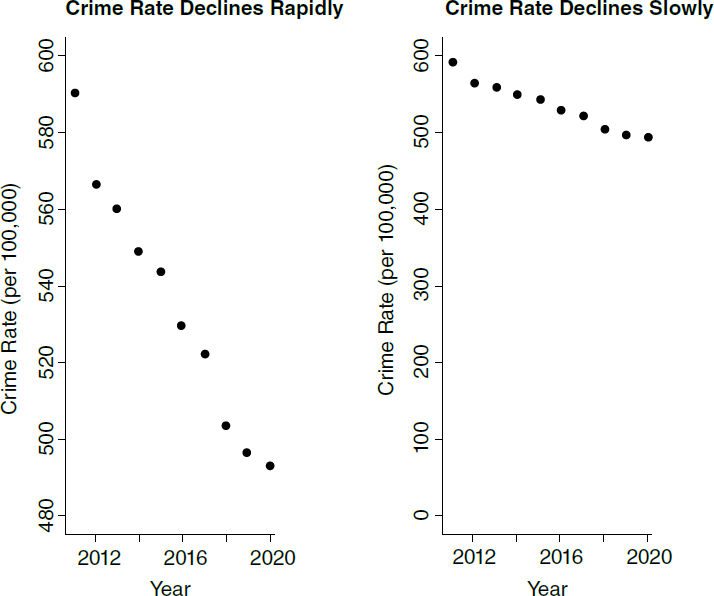
2011 through 2020; in Figure 2, the same rate appears to drop slowly.94 The moral is simple: Pay attention to the markings on the axes to determine whether the scale is appropriate. A similar admonition applies to bar charts, which display counts or rates across categories.95
How Are Distributions Displayed?
A graph commonly used to display the distribution of data is the histogram. One axis denotes the numbers, and the other indicates how often these numbers fall within specified intervals (called “bins” or “class intervals”). For example, we
94. Florida Statistical Analysis Center, Florida Dep’t of Law Enforcement, Statewide Reported Domestic Violence Offenses in Florida, 1992–2020, https://perma.cc/KQ7F-H6UM. The data are from the Florida Uniform Crime Report statistics on crimes ranging from simple stalking and forcible fondling to murder and arson.
95. See David Spiegelhalter, The Art of Statistics: Learning from Data 25–26 (2019) (for an example using survival rates of patients admitted to different hospitals).
flipped a quarter 10 times in a row and counted the number of heads in this “batch” of 10 tosses. Repeating this exercise until we obtained 50 batches, we recorded the following counts:96
![]()
The histogram is shown in Figure 3.97 A histogram displays how the data are distributed over the range of possible values. The spread can be made to appear larger or smaller, however, by changing the scale of the horizontal axis. Likewise, the shape can be altered somewhat by changing the size of the bins. It may be worth inquiring how the analyst chose the bin widths. As the width of the bins decreases, the graph becomes more detailed, but the appearance becomes

96. The coin landed heads 7 times in the first 10 tosses; by coincidence, there were also 7 heads in the next 10 tosses; there were 5 heads in the third batch of 10 tosses; and so forth.
97. In Figure 3, the bin width is 1. There were no 0’s or 1’s in the data, so the bars over 0 and 1 disappear. There is a bin from 1.5 to 2.5; the four 2’s in the data fall into this bin, so the bar over the interval from 1.5 to 2.5 has height 4. There is another bin from 2.5 to 3.5, which catches five 3’s; the height of the corresponding bar is 5. And so forth. Five is the most likely count in any random batch, but in these 50 batches, a count of 4 heads occurred more frequently, as shown by the larger height for bin 4.
All the bins in Figure 3 have the same width, so this histogram is just like a bar graph. However, data are often published in tables with unequal intervals. The resulting histograms will have unequal bin widths; bar heights should be calculated so that the areas (height × width) are proportional to the frequencies. In general, a histogram differs from a bar graph in that it represents frequencies by area, not height. See Freedman et al., supra note 14, at 31–41.
more ragged until finally the graph is effectively a plot of each datum. The optimal bin width depends on the subject matter and the goal of the analysis.
Is an Appropriate Measure Used for the Center of a Distribution?
Perhaps the most familiar descriptive statistic is the mean (or “arithmetic mean”). The mean can be found by adding all the numbers and dividing the total by how many numbers were added. By comparison, the median cuts the numbers into halves: half the numbers are larger than the median and half are smaller.98 Yet a third statistic is the mode, which is the most common number in the dataset. These statistics are different, although they are not always clearly distinguished. In ordinary language, the arithmetic mean, the median, and the mode seem to be referred to interchangeably as “the average.” In statistical parlance, however, the average is the arithmetic mean. The mode is rarely used by statisticians, because it is unstable: Small changes to the data often result in large changes to the mode. The mean takes account of all the data—it involves the total of all the numbers; however, particularly with small datasets, a few unusually large or small observations may have too much influence on the mean. The median is resistant to such outliers.
Studies of damage awards in tort cases find that the mean is larger than the median.99 This is because the mean takes into account (indeed, is heavily influenced by) the magnitudes of the relatively few very large awards, whereas the median is influenced only by the number of such awards. If one is seeking a single, representative number for the awards, the median may be more useful than the mean.100 Still, if the issue is whether insurers were experiencing more
98. Technically, at least half the numbers are at the median or larger; at least half are at the median or smaller. When the distribution is symmetric, the mean equals the median. The values diverge, however, when the distribution is asymmetric, or skewed.
99. Herbert M. Kritzer et al., An Exploration of “Noneconomic” Damages in Civil Jury Awards, 55 Wm. & Mary L. Rev. 971 (2014) (summarizing empirical research); Thomas H. Cohen & Steven K. Smith, U.S. Dep’t of Justice, Bureau of Justice Statistics Bulletin NCJ 202803, Civil Trial Cases and Verdicts in Large Counties 2001, 10 (2004) (in a probability sample of cases, the median compensatory award in wrongful death cases was $961,000, whereas the mean award was around $3.75 million for the 162 cases in which the plaintiff prevailed); cf. Stephen J. Choi & Theodore Eisenberg, Punitive Damages in Securities Arbitration: An Empirical Study, 39 J. Legal Stud. 497, 513 tbl. 1 (2010) (reporting much higher mean than median arbitration awards). In TXO Production Corp. v. Alliance Resources Corp., 509 U.S. 443 (1993), briefs portraying the punitive damage system as out of control pointed to mean punitive awards. These were some 10 times larger than the median awards described in briefs defending the system of punitive damages. Michael Rustad & Thomas Koenig, The Supreme Court and Junk Social Science: Selective Distortion in Amicus Briefs, 72 N.C. L. Rev. 91, 145–47 (1993).
100. E.g., Heinrich v. Sweet, 308 F.3d 48 (1st Cir. 2002) (two outliers made the median survival time a better indicator of what might have happened had a patient not undergone
costs from jury verdicts, the mean is the more appropriate statistic: The total of the awards is directly related to the mean, not to the median.101
Research also has shown considerable stability in the ratio of punitive to compensatory damage awards, and the Supreme Court has placed great weight on this ratio in deciding whether punitive damages are excessive in a particular case. In Exxon Shipping Co. v. Baker,102 Exxon contended that an award of $2.5 billion in punitive damages for a catastrophic oil spill in Alaska was unreasonable under federal maritime law. The Court looked to a “comprehensive study of punitive damages awarded by juries in state civil trials [that] found a median ratio of punitive to compensatory awards of just 0.62:1, but a mean ratio of 2.90:1.”103 The higher mean could be the result of some large and atypical punitive awards.104 Looking to the median ratio as “the line near which cases like this one largely should be grouped,” the majority concluded that “a 1:1 ratio, which is above the median award, is a fair upper limit in such maritime cases [of reckless conduct].”105
Is an Appropriate Measure of Variability Used?
The location of the center of a batch of numbers reveals nothing about the variations exhibited by these numbers. The numbers 1, 2, 5, 8, 9 have 5 as their mean and median. So do the numbers 5, 5, 5, 5, 5. In the first batch, the numbers vary considerably about their mean; in the second, the numbers do not vary at all.
experimental therapy). In passing on proposed settlements in class-action lawsuits, courts have been advised to look to the magnitude of the settlements negotiated by the parties. But the mean settlement will be large if a higher number of meritorious, high-cost cases are resolved early in the life cycle of the litigation. This possibility led the court in In re Educational Testing Service Praxis Principles of Learning and Teaching, Grades 7–12 Litigation, 447 F. Supp. 2d 612, 625 (E.D. La. 2006), to regard the smaller median settlement as “more representative of the value of a typical claim than the mean value” and to use this median in extrapolating to the entire class of pending claims.
101. To get the total award, just multiply the mean by the number of awards; by contrast, the total cannot be computed from the median. (The more pertinent figure for the insurance industry is not the total of jury awards, but actual claims experience including settlements; of course, even the risk of large punitive damage awards may have considerable impact.)
102. 554 U.S. 471 (2008).
103. Id. at 499.
104. According to the Court, “the outlier cases subject defendants to [disproportionate] punitive damages,” id. at 500, and the “stark unpredictability” of these rare awards is the “real problem.” Id. at 499. This perceived unpredictability has been the subject of various statistical studies and much debate. See Theodore Eisenberg et al., Variability in Punitive Damages: Empirically Assessing Exxon Shipping Co. v. Baker, 166 J. Institutional & Theoretical Econ. 5 (2010) (also criticizing the use of a constant 1:1 ratio across the entire range of damage awards); Anthony J. Sebok, Punitive Damages: From Myth to Theory, 92 Iowa L. Rev. 957 (2007).
105. 554 U.S. at 513.
Statistical measures of variability include the range, the interquartile range, and the standard deviation. The range is the difference between the largest number in the batch and the smallest. The range seems natural, and it indicates the maximum spread in the numbers, but the range is unstable because it depends entirely on the most extreme values.
The interquartile range is the difference between the 25th and 75th percentiles. By definition, 25% of the data fall below the 25th percentile, 90% fall below the 90th percentile, and so on. The median is the 50th percentile. The interquartile range contains 50% of the numbers and is resistant to changes in extreme values.
The standard deviation can be viewed as a kind of average or typical deviation from the mean.106 Suppose we have a batch of 50 numbers whose mean is 100. The standard deviation is found by subtracting this mean from each number, squaring each of these deviations, adding up the squared deviations, dividing by 50 (to get the mean squared deviation, or “variance”), and taking the square root. For example, if one of the numbers is 105, then it deviates from the mean by 5, and the square of 5 is 52 = 25. If the mean of all such squared deviations is 400, then the standard deviation is the square root of 400, which is 20. Taking the square root gets back to the original scale of the measurements. For example, if the numbers are measurements of length in inches, the mean and standard deviation are also in inches.
There are no hard and fast rules about which statistic is the best. In general, the bigger the measures of spread are, the more the numbers are dispersed.107 Particularly in small datasets, the standard deviation can be influenced heavily by a few outlying values. To assess the extent of this influence, the mean and the standard deviation can be recomputed with the outliers discarded. These “trimmed” statistics (and some others) are more robust (less sensitive to outliers). Beyond this, any of the statistics can (and often should) be supplemented with a diagram that displays much of the data.
106. When the distribution follows the normal curve, about 68% of the data will lie within plus-or-minus 1 standard deviation of the mean; about 95% will lie within 2 standard deviations of the mean. For other distributions, the proportions will be different.
107. In Exxon Shipping Co. v. Baker, 554 U.S. 471 (2008), along with the mean and median ratios of punitive to compensatory awards of 0.62 and 2.90, the Court referred to a standard deviation of 13.81. Id. at 499. These numbers led the Court to remark that “[e]ven to those of us unsophisticated in statistics, the thrust of these figures is clear: the spread is great, and the outlier cases subject defendants to punitive damages that dwarf the corresponding compensatories.” Id. at 500. The size of the standard deviation compared to the mean supports the observation that ratios in the cases of jury award studies are dispersed. A graph of each pair of punitive and compensatory damages offers more insight into how scattered these figures are. See Theodore Eisenberg et al., The Predictability of Punitive Damages, 26 J. Legal Stud. 623 (1997), and the section titled “Scatter Diagrams” below.
What Inferences Can Be Drawn from the Data?
The inferences that may be drawn from a study depend on the design of the study and the quality of the data (see section titled “How Have the Data Been Collected?” above). The data might not address the issue of interest, might be systematically in error, or might be difficult to interpret because of confounding. Statisticians would group these concerns together under the rubric of “bias.” In this context, bias means systematic error, with no connotation of prejudice. We turn now to another concern, namely, the impact of random chance on study results. This contribution to total error may be called random error, sampling error, chance error, or statistical error.108
If a pattern in the data is the result of chance, it is likely to wash out when more data are collected. By applying the laws of probability, a statistician can assess the likelihood that random error will create spurious patterns of certain kinds. Such assessments are often viewed as essential when making inferences from data. Thus, statistical inference typically involves tasks such as the following, which will be discussed in the rest of this guide.
- Estimation. A statistician draws a sample from a population (see section titled “Descriptive Surveys and Censuses” above) and estimates a parameter—that is, a numerical characteristic of the population. Random error will throw the estimate off the mark. The question is, by how much? The precision of an estimate is usually reported in terms of the standard error and a confidence interval.
- Significance testing. A “null hypothesis” is formulated—for example, that a parameter takes a particular value. Because of random error, an estimated value for the parameter is likely to differ from the value specified by the null—even if the null is right. (“Null hypothesis” is often shortened to “null.”) How likely is it to get a difference as large as, or larger than, the one observed in the data? This chance is known as a p-value. Small p-values argue against the null hypothesis as such values suggest the observed difference is not likely due to chance alone. Statistical significance can be determined by reference to the p-value; significance testing is the technique for computing p-values and determining statistical significance. Significance testing is sometimes called hypothesis testing; some statisticians
108. Econometricians use the parallel concept of random disturbance terms. See Rubinfeld & Card, supra note 25. Randomness and cognate terms have precise technical meanings; it is randomness in the technical sense that justifies the probability calculations behind standard errors, confidence intervals, and p-values (see section titled “What Does It Mean to Be Random?” above and the sections titled “Estimation” and “p-values, Significance Levels, and Hypothesis Tests” below). For a discussion of samples and populations, see section titled “Descriptive Surveys and Censuses” above.
- restrict the latter term to instances in which there are two explicit hypotheses to be addressed.109
- Developing a statistical model. Statistical inferences often depend on the validity of statistical models for the data. If the data are collected on the basis of a probability sample or a randomized experiment, there will be statistical models that suit the occasion, and inferences based on these models will be secure. Otherwise, calculations are generally based on analogy: This group of people is like a random sample; that observational study is like a randomized experiment. The fit between the statistical model and the data-collection process may then require examination—how good is the analogy? If the model breaks down, that will bias the analysis.
- Computing posterior probabilities. Given the sample data, what is the probability that a particular hypothesis about the population (such as the null hypothesis in a significance test) is true? The question might be of direct interest to the courts, especially when translated into English; for example, the null hypothesis might be that African-American and white job applicants have the same probability of passing a qualifying examination—in other words, the test does not adversely impact one group. Posterior probabilities can be computed using a formula called Bayes’ rule.110
109. As explained in the section titled “p-values, Significance Levels, and Hypothesis Tests” below, tests of significance focus on the degree to which data are inconsistent with a specified null hypothesis. There is no explicit alternative hypothesis, although frequently an alternative is implicit in the choice to use a one-sided or two-sided test. The p-value is the probability that data as or more unexpected than the data observed would occur by chance under the null hypothesis. The statistical significance of the result is assessed in terms of the p-value. Sir Ronald Fisher usually is credited with introducing this framework. But see Michael Cowles & Caroline Davis, On the Origins of the .05 Level of Statistical Significance, 37 Am. Psych. 553 (1982).
By contrast, formal hypothesis testing (as developed by Jerzy Neyman and Egon Pearson) requires explicit specification of an alternative hypothesis and then development of a test procedure with pre-specified probabilities of making two types of errors—type I (rejecting the null hypothesis when it is true) and type II (failing to reject the null hypothesis when the alternative is true). The end result here is a decision rather than a p-value. The two procedures end up being closely related in practice despite their philosophical differences. See, e.g., Erich L. Lehmann, The Fisher, Neyman-Pearson Theories of Testing Hypotheses: One Theory or Two?, 88 J. Am. Stat. Ass’n 1242 (1993), https//doi.org/10.2307/2291263.
110. The theorem is named after the Reverend Thomas Bayes (England, c. 1701–1761). An elementary version of the rule is derived in the Appendix. Bayes’ essay on the subject was published after his death: An Essay Toward Solving a Problem in the Doctrine of Chances, 53 Phil. Trans. Royal Soc’y London 370 (1763–1764). On the foundations and varieties of Bayesian and other forms of statistical inference, see, for example, Richard M. Royall, Statistical Inference: A Likelihood Paradigm (1997); David Freedman, Some Issues in the Foundation of Statistics, 1 Found. Sci. 19 (1995), reprinted in Topics in the Foundation of Statistics 19 (Bas C. van Fraasen ed., 1997); Hal S. Stern, Comparing Philosophies of Statistical Inference, in Handbook of Forensic Statistics 91 (David Banks et al. eds., 2021); see also David H. Kaye, What Is Bayesianism? in Probability and Inference in the Law of Evidence: The Uses and Limits of Bayesianism (Peter Tillers & Eric Green eds., 1988), reprinted in
Key ideas of estimation and testing will be illustrated by courtroom examples, with some complications and mathematical details omitted for ease of presentation.111 Bayesian reasoning with regard to forensic-science testimony is discussed in the Appendix.
The first example, on estimation, concerns the Presidential Recordings and Materials Preservation Act of 1974, which impounded President Richard Nixon’s presidential papers after he resigned.112 Nixon sued, seeking compensation on the theory that the materials belonged to him personally. Courts ruled in his favor: Nixon was entitled to the fair market value of the papers, with the amount to be proved at trial.113
The Nixon papers were stored in 20,000 boxes at the National Archives in Alexandria, Virginia. It was plainly impossible to value this entire population of material. Appraisers for the plaintiff therefore took a random sample of 500 boxes. (From this point on, details are simplified; thus, the example becomes somewhat hypothetical.) The appraisers determined the fair market value of each sample box. The average of the 500 sample values turned out to be $2,000. The standard deviation (see section titled “Is an Appropriate Measure of Variability Used?” above) of the 500 sample values was $2,200. Many boxes had low appraised values, whereas some boxes were considered to be extremely valuable; this spread explains the large standard deviation.
Estimation
What Estimator Should Be Used?
With the Nixon papers, it is natural to use the average value of the 500 sample boxes to estimate the average value of all 20,000 boxes comprising the population. With the average value for each box having been estimated as $2,000, the plaintiff demanded compensation in the amount of 20,000 × $2,000 = $40,000,000.
In more complex problems, statisticians may have to choose among several estimators. Generally, estimators that tend to make smaller (or less costly) errors are preferred; however, “error” (or the losses that result from errors) might be quantified in more than one way. Moreover, the advantage of one estimator over another may depend on features of the population that are largely unknown, at least before the data are collected and analyzed. For complicated problems,
28 Jurimetrics J. 161 (1988) (distinguishing between “Bayesian probability,” “Bayesian statistical inference,” “Bayesian inference writ large,” and “Bayesian decision theory”).
111. Some technical details appear in the appendices to David H. Kaye & David A. Freedman, Reference Guide on Statistics, in Reference Manual on Scientific Evidence (3d ed. 2011).
112. 44 U.S.C. § 2111.
113. Nixon v. United States, 978 F.2d 1269 (D.C. Cir. 1992); Griffin v. United States, 935 F. Supp. 1 (D.D.C. 1995).
professional skill and judgment may therefore be required when choosing a sample design and an estimator. In such cases, the choices and the rationale for them should be documented.
What Is the Standard Error?
An estimate based on a sample is likely to be off the mark, at least by a small amount, because of random error. The standard error gives the likely magnitude of this random error, with smaller standard errors indicating better estimates.114 In our example of the Nixon papers, the standard error for the sample average can be computed from (1) the size of the sample—500 boxes—and (2) the standard deviation of the sample values. Bigger samples give estimates that are more precise. Accordingly, the standard error should go down as the sample size grows, although the rate of improvement slows as the sample gets bigger. (“Sample size” and “the size of the sample” just mean the number of items in the sample; the “sample average” is the average value of the items in the sample.) The standard deviation of the sample comes into play by measuring heterogeneity. The less heterogeneity in the values, the smaller the standard error. For example, if all the values were about the same, a tiny sample would give an accurate estimate. Conversely, if the values are quite different from one another, a larger sample would be needed.
With a random sample of 500 boxes and a standard deviation of $2,200, the standard error for the sample average is estimated to be about $100.115 The plaintiff’s total demand was figured as the number of boxes (20,000) times the sample average ($2,000), or $40,000,000. Therefore, the standard error for the total
114. We distinguish between (1) the standard deviation of the sample data, which measures the spread in the sample values, and (2) the standard error of the sample average, which measures the likely size of the random error in the sample average. Generally, the standard error of an estimator (such as the sample average) is the standard deviation of that estimator as applied to (hypothetically) repeated samples. Courts typically use the broader term “standard deviation” when referring to the standard error. E.g., Castaneda v. Partida, 430 U.S. 482 (1977).
115. The standard error for the sample average equals
. Freedman et al., supra note 14, at 367–70. N stands for the size of the population, which is 20,000; n stands for the size of the sample, which is 500. The first factor, with the N’s in it, is the finite sample correction factor. Here, as in many other such examples, the correction factor is so close to 1 that it can safely be ignored. (This is why the size of population usually has no bearing on the precision of the sample average as an estimator for the population average.) Next, σ is the population standard deviation. Its value is unknown but can be estimated by the sample standard deviation of $2,200. The standard error for the sample mean is therefore estimated from the data as $2,200/√500, which is nearly $100.
demand is 20,000 times the standard error for the sample average: 20,000 × $100 = $2,000,000.116
How is the standard error to be interpreted? Just by the luck of the draw, a few too many high-value boxes may have come into the sample, in which case the estimate of $40,000,000 is too high. Or, a few too many low-value boxes may have been drawn, in which case the estimate is too low. This is random error. The net effect of random error is unknown, because data are available only on the sample, not on the full population. However, the net effect is likely to be something close to the standard error of $2,000,000. Random error throws the estimate off, one way or the other, by something close to the standard error. The role of the standard error is to gauge the likely size of the random error.
The plaintiff’s argument may be open to a variety of objections, particularly regarding appraisal methods. However, the sampling plan is sound, as is the extrapolation from the sample to the population. And there is little need for a larger sample: Relative to the total claim of $40 million, a standard error of $2 million is reasonably small.
What Is the Confidence Interval?
Although random errors larger in magnitude than the standard error are commonplace, random errors larger in magnitude than two or three times the standard error are unusual. Confidence intervals make these ideas more precise. Usually, a confidence interval for the population average (the average of all the values in the population) is centered at the sample average; the desired confidence level is obtained by adding and subtracting a suitable multiple of the standard error. In dealing with large samples, statisticians who say that the population average falls within 1 standard error of the sample average will be correct about 68% of the time. Those who say “within 2 standard errors” will be correct about 95% of the time, and those who say “within 3 standard errors” will be correct about 99.7% of the time, and so forth.
The normal curve and large samples
These confidence levels correspond to areas under a famous bell-shaped curve—the normal curve. According to a fundamental theorem of statistics (the central
116. We are assuming a simple random sample. Generally, the formula for the standard error must take into account the method used to draw the sample and the nature of the estimator. In fact, the Nixon appraisers used more elaborate statistical procedures. Moreover, they valued the material as of 1995, extrapolated backward to the time of taking (1974), and then added interest. After 20 years of litigation, Nixon’s estate settled with the government for $18 million. U.S. Dep’t of Just., Press Release, June 12, 2000, https://perma.cc/PJC9-47CY.
limit theorem), if we were to draw not merely a single large sample from a much larger population, or even 500 of them as in the Nixon example, but millions upon millions of them (replacing the items from each sample before drawing the next one), and if we then sorted the sample averages into appropriate bins of a histogram, the heights of the bins would be greatest near the population average, and they would fall off symmetrically on each side as prescribed by the values of the normal curve centered at this point and having a standard deviation that is the standard error.117
The confidence interval relies on this understanding of the distribution of sample means but goes in the other direction. Knowing how the sample statistic behaves as a function of the population parameters, we draw an interval around the sample statistic that we hope will cover the true value (the parameter). The mathematical properties of the normal distribution justify the numbers used to express the “confidence.”118 In particular,
- To get a 68% confidence interval, start at the sample average, then add and subtract 1 standard error.
- To get a 95% confidence interval, start at the sample average, then add and subtract twice the standard error.
- To get a 99.7% confidence interval, start at the sample average, then add and subtract three times the standard error.
With the Nixon papers, the 68% confidence interval for plaintiff’s total demand runs
- from $40,000,000 − $2,000,000 = $38,000,000
- to $40,000,000 + $2,000,000 = $42,000,000.
117. The normal curve is the density of a normal distribution. The distribution has two parameters—the population mean (often denoted µ) and the standard deviation (σ), which is the standard error of the variable x (here, the sample mean, which varies from one sample to the next). The equation is
where e = 2.71828 . . . and π = 3.14159. . . . Once the two parameters µ and σ are given, the density is completely specified.
118. The area under the normal curve between x = µ−σ and x = µ+σ is close to 68.3%. Likewise, the area between µ−2σ and µ+2σ is close to 95.4%. Many academic statisticians would use ±1.96 SE for a 95% confidence interval. However, the normal curve only gives an approximation to the relevant chances, and the error in that approximation will often be larger than a few tenths of a percent. For simplicity, we use ±1 SE for the 68% confidence level, and ±2 SE for 95% confidence.
The 95% confidence interval runs
- from $40,000,000 − (2 × $2,000,000) = $36,000,000
- to $40,000,000 + (2 × $2,000,000) = $44,000,000.
The 99.7% confidence interval runs
- from $40,000,000 − (3 × $2,000,000) = $34,000,000
- to $40,000,000 + (3 × $2,000,000) = $46,000,000.
To write this more compactly, we abbreviate standard error as SE. Thus, 1 SE is one standard error, 2 SE is twice the standard error, and so forth. With a large sample and an estimate like the sample average, a 68% confidence interval ranges from
estimate − 1 SE to estimate + 1 SE.
A 95% confidence interval is ranges from
estimate − 2 SE to estimate + 2 SE.
A 99.7% confidence interval ranges from
estimate − 3 SE to estimate + 3 SE.
For a given sample size, increased confidence can be attained only by widening the interval. The 95% confidence level is the most popular, but some authors use 99%, and 90% is seen on occasion. (The corresponding multipliers on the SE are about 2, 2.6, and 1.6, respectively.) The phrase “margin of error” generally means twice the standard error. In medical journals, “confidence interval” is often abbreviated as “CI.” The relationship between width and confidence is shown in Figure 4.

The picture shows a tradeoff between precision (the width of the interval) and confidence (that the interval covers the actual population value). In sum, an estimate based on a sample will differ from the exact population value, because of random error. The standard error gives the likely size of the random error. If the standard error is small, random error probably has little effect. If the standard error is large, the estimate may be far away from the population value. Confidence intervals are a technical refinement that provides a formalism for assessing the impact of random error or chance variation on the estimate.
Other situations
Intervals based on the standard error, with confidence levels read off the normal curve, are appropriate for estimators that are essentially unbiased and obey the central limit theorem. They generally work for sums, averages, and rates, although much depends on the design of the sampling and other matters. CIs determined via the normal curve may not work well as estimates of extremely small quantities. Table 1 of the section titled “Is the Measurement Process Valid?” presents an extreme example. The table showed that toolmark examiners given 30 pairs of cartridges from ammunition fired from the same guns and 45 pairs from different guns correctly classified every pair according to the true source. But what if the same examiners had been brought back for a second experiment with the same cartridge cases (and with no memory of the first experiment)? Would they have done as well? What about a third experiment? It would be extraordinary if they never erred in one experiment after another ad infinitum. Perhaps we can think of the one experiment as if it were a random sample from an infinite population of repeated experiments. Given this framework, we might want a confidence interval that will estimate the proportion of false-positive errors on the part of the examiners in an infinite stream of experiments with guns and ammunition exactly like those in the study. The observed proportion of errors in the one experiment is zero, which makes the plug-in estimate of the standard error zero as well. However, a confidence interval of zero width cannot be right. The probability of false-positive errors could be higher than zero, and an examiner could still get all 45 determinations for the false pairs correct. The problem is that because every determination in the sample (the one experiment) is correct, there is no variability to inform what we might see in future samples (experiments).
How should we proceed? It is easy to show that an interval from 0 to 6.5% would achieve at least 95% “confidence.”119 So if we are willing to embrace anything in the range of 0 to 6.5% as the true error-rate when given samples with an
119. When the long-run false-positive error rate is 6.5%, the probability of 45 independent correct classifications of cartridges from different pairs of guns is (1−0.065)45 = 0.049. When the “true” error rate is greater than 6.5%, that probability for zero errors in the sample is smaller still.
observed rate of 0/45, we will be correct at least 95% of the time (in the long run). But this interval is a very conservative estimate. How to construct a confidence or other interval for the probability of an event when 0/n are observed goes by the name of the zero-numerator problem, and several approaches have been proposed.120
In still other situations (for example, where observations are dependent), other methods can be used to obtain confidence intervals. One class of methods repeatedly resamples from the observed data to approximate what would happen in repeated samples from the full population.121 With modern computers, the resulting bootstrap confidence intervals are enticingly easy to calculate, but they too require certain assumptions to be verified.122
How Big Should the Sample Be?
There is no easy answer to this sensible question. Much depends on the level of error that is tolerable, the material being sampled, and the sampling method. Increasing the size of the sample provides no protection against bias (“nonsampling error”). Indeed, beyond some point, large samples are harder to manage and more vulnerable to nonsampling error. To reduce bias, the researcher must improve the design of the study or use a statistical model more tightly linked to the data-collection process. Larger samples generally will reduce the level of random error (“sampling error”). It rarely will be sensible to draw a probability sample with fewer than, say, two or three dozen items, and with such small samples, methods based solely on the normal curve (see section titled “What Is the Standard Error?” above) will not apply. A pilot sample is often valuable, partly to obtain an initial estimate of characteristics of the population that may be used in
120. E.g., Noriah M. Al-Kandari & Paul H. Garthwaite, Bayesian Analysis of Misclassified Binomial Data: Double-Sampling and the Zero-Numerator Problem, Communications in Statistics—Simulation & Computation (2020), https://doi.org/10.1080/03610918.2020.1855448; B. D. Jovanovic & P. S. Levy, A Look at the Rule of Three, 51 Am. Statistician 137 (1997); Robert L. Winkler et al., The Role of Informative Priors in Zero-Numerator Problems: Being Conservative Versus Being Candid, 56 Am. Statistician 1 (2002).
121. See, e.g., Freedman, supra 25, at 147–50; David H. Kaye, Frequentist Statistical Inference, in Handbook of Forensic Statistics 39, 66–68 (David Banks et al. eds., 2021) (discussing the basic idea). On the patentability of procedures relying on bootstrapping or other resampling methods, see SAP America v. InvestPic, 898 F.3d 1161 (Fed. Cir. 2018) (investment analysis); Cybergenetics Corp. v. Inst. of Env’l Sci. & Rsch., 490 F. Supp. 3d 1237 (N.D. Ohio 2020) (in discerning separate contributors to DNA mixtures), aff’d, 856 Fed. App’x 312 (Fed. Cir. 2021).
122. See In re Sonic Corp. Customer Data Sec. Breach Litig., No. 1:17-md-2807, MDL No. 2807, 2021 WL 5916743 (N.D. Ohio Dec. 15, 2021) (bootstrap estimate that losses to credit-card companies from a computer security breach exceeded $76,000,000 were inadmissible because the bootstrap sample was small and unrepresentative); Bradley Efron & Robert J. Tibshirani, An Introduction to the Bootstrap (1994); Freedman, supra note 25, at 150.
determining the final sample size.123 If a population appears to be heterogeneous, then alternatives to simple random sampling, such as stratified random samples (that are each fairly homogeneous), may provide more representative samples and more precise estimates for the same total sample size. As these examples illustrate, probability samples require some effort in the design phase.
Population size (i.e., the number of items in the population) usually has little bearing on the precision of estimates for the population average. This is surprising. On the other hand, population size has a direct bearing on estimated totals. Both points are illustrated by the Nixon papers (see section titled “What Is the Standard Error?” above). To be sure, drawing a probability sample from a large population may involve a lot of work. Samples presented in the courtroom have ranged from 5 (tiny) to 1.7 million (huge).124
What Are the Technical and Interpretive Difficulties with Confidence Intervals?
To begin with, “confidence” has an esoteric meaning in this context. The confidence level indicates the percentage of the time that intervals from repeated samples would cover the true value. The confidence level does not express the chance that repeated estimates would fall into the stated confidence interval.125
123. Suppose a researcher is interested in the association between alcohol intoxication and single-vehicle accidents. A small sample of accident records (along with intuitions) could suggest some guess for the population proportion of single-vehicle crashes in which the driver was found to be intoxicated. Assume the guess is 50%. Suppose further that the researcher is willing to tolerate errors of up to ±3% in the estimate from the larger sample being planned. Finally, suppose that the researcher plans to report a conventional 95% confidence interval. It can be shown that a simple random sample of approximately 1,067 single-vehicle accident records should suffice. Hence, the researcher collects 1,067 records at random and determines the proportion in which intoxication was in the accident record. The observed proportion in this sample might be 40% or 0.4, to pick a concrete number. The earlier guess of 50% no longer matters—it was just used to get a sense of the sample size for the full study, and the researcher now can report a 95% CI from the full study. The estimate becomes .40 ± 1.96 =.40 ± .03, which is about 37% to 43%.
124. Lebrilla v. Farmers Grp., Inc., No. 00-CC-017185 (Cal. Super. Ct., Orange Cnty., Dec. 5, 2006) (preliminary approval of settlement). This was a class action lawsuit on behalf of plaintiffs who were insured by Farmers and had automobile accidents. Plaintiffs alleged that replacement parts recommended by Farmers did not meet specifications: Small samples were used to evaluate these allegations. At the other extreme, it was proposed to adjust Census 2000 for undercount and overcount by reviewing a sample of 1.7 million persons. See Brown et al., supra note 36, at 353.
125. Opinions reflecting this misinterpretation include Turpin v. Merrell Dow Pharm., Inc., 959 F.2d 1349, 1353 (6th Cir. 1992) (“If a confidence interval of ‘95 percent between 0.8 and 3.10’ is cited, this means that random repetition of the study should produce, 95 percent of the time, a relative risk somewhere between 0.8 and 3.10.”); Garcia v. Tyson Foods, Inc., 890 F. Supp. 2d 1273, 1285 (D. Kan. 2012) (“Dr. Radwin testified that his study was conducted within a confidence interval of 95—that is ‘if I did this study over and over again, 95 out of a hundred times I would
With the Nixon papers, the 95% confidence interval should not be interpreted as saying that 95% of all random samples will produce estimates in the range from $36 million to $44 million. Rather, a high degree of “confidence” makes it reasonable to accept the one sample interval as a plausible statement of what the value of all the papers could be.
Second, the confidence level does not give the probability that the unknown parameter lies within the confidence interval.126 For example, the 95% confidence level should not be translated to a 95% probability that the total value of the papers is in the range from $36 million to $44 million. According to the frequentist theory of statistics, probability statements cannot be made about population characteristics: Probability statements apply to the behavior of samples. That is why the different term “confidence” is used.
Third, this “confidence” is a statement about the entire region. One might think that values near the center of the interval are more likely to be closer to the true value than those at the extremes. Yet the statement of confidence applies equally to all the values in the interval. Moreover, that the intervals have sharp boundaries does not imply that there is an important difference between a value at the edge of the interval and one just beyond it.
expect to get an average between that interval.’”); In re Silicone Gel Breast Implants Prods. Liab. Litig., 318 F. Supp. 2d 879, 897 (C.D. Cal. 2004) (“a margin of error between 0.5 and 8.0 at the 95% confidence level . . . means that 95 times out of 100 a study of that type would yield a relative risk value somewhere between 0.5 and 8.0”).
Language from another reference guide in the previous edition of this Reference Manual that is often quoted may inadvertently convey the incorrect impression that a confidence coefficient such as 95% refers to the percentage of results in (hypothetically) repeated studies that would be expected to lie within the interval reported in the study before the court. See, e.g., Rhyne v. U.S. Steel Corp., 474 F. Supp. 3d 733, 744 (W.D.N.C. 2020) (“‘If a 95% confidence interval is specified, the range encompasses the results we would expect 95% of the time if samples for new studies were repeatedly drawn from the population.’ Reference Guide on Epidemiology, at 580.”). However, simulations suggest that the confidence coefficient for a sample mean from a normal population tends to overstate the probability that the next sample mean will lie within the interval. Geoff Cumming & Robert Maillardet, Confidence Intervals and Replication: Where Will the Next Mean Fall?, 11 Psych. Methods 217 (2006), https://doi.org/10.1037/1082-989X.11.3.217 (finding that “[o]n average, a 95% CI will include just 83.4% of future replication means”). The more technically correct statement in the Silicone Gel case would be that “the confidence interval of 0.5 to 8.0 means that the relative risk in the population plausibly could fall within this wide range—and that in roughly 95 times out of 100 random samples from the same population, the confidence intervals (however wide they might be) would include the population value (whatever it is).”
126. See, e.g., Freedman et al., supra note 14, at 383–86. Consequently, it is misleading to suggest that “[t]he confidence interval means . . . it is 95 percent likely that the actual [value of the parameter being estimated] is somewhere in the interval, somewhere between the low end of the interval and its high end,” Center for Biological Diversity v. U.S. Fish & Wildlife Serv., 342 F. Supp. 3d 968, 977 (N.D. Cal. 2018), or that “a 95-percent median confidence interval of 89.43 to 90.28 percent [means] that the true median is 95-percent likely to fall within that range,” Cnty. of Douglas v. Nebraska Tax Equalization & Rev. Comm’n, 894 N.W.2d 308, 316 (Neb. 2017).
Fourth, for a given confidence level, a narrower interval indicates a more precise estimate, whereas a broader interval indicates less precision.127 A high confidence level with a broad interval means very little, but a high confidence level for a small interval is impressive, indicating that the random error in the sample estimate is low. For example, take a 95% confidence interval for a damage claim. An interval that runs from $36 million to $44 million is more precise than a much wider interval that goes from $10 million to $70 million. Statements about confidence without mention of an interval are practically meaningless.128
The final point to make is that standard errors and confidence intervals are often derived from statistical models for the process that generated the data. The model usually has parameters—numerical constants describing the population from which samples were drawn. When the values of the parameters are not known, the statistician must work backwards, using the sample data to make estimates. That was the case for valuing the Nixon papers. One parameter is the average value of all 20,000 boxes, and another parameter is the standard deviation of the 20,000 values.129 Generally, the probabilities used in drawing inferences are computed from a model with estimated parameter values.
127. See section titled “What Is the Standard Error?” above. In Cimino v. Raymark Industries, Inc., 751 F. Supp. 649 (E.D. Tex. 1990), rev’d, 151 F.3d 297 (5th Cir. 1998), the district court drew certain random samples from more than 6,000 pending asbestos cases, tried these cases, and used the results to estimate the total award to be given to all plaintiffs in the pending cases. The court then held a hearing to determine whether the samples were large enough to provide accurate estimates. The court’s expert, an educational psychologist, testified that the estimates were accurate because the samples matched the population on such characteristics as race and the percentage of plaintiffs still alive. Id. at 664. However, the matches occurred only in the sense that population characteristics fell within 99% confidence intervals computed from the samples. The court thought that matches within the 99% confidence intervals proved more than matches within 95% intervals. Id. This is backward. To be correct in a few instances with a 99% confidence interval is not very impressive—by definition, such intervals are broad enough to ensure coverage approximately 99% of the time.
128. In Hilao v. Estate of Marcos, 103 F.3d 767 (9th Cir. 1996), “an expert on statistics . . . testified that . . . a random sample of 137 claims would achieve ‘a 95% statistical probability that the same percentage determined to be valid among the examined claims would be applicable to the totality of [9,541 facially valid] claims filed.’” Id. at 782. There is no 95% “statistical probability” that a percentage computed from a sample will be “applicable” to a population. One can compute a confidence interval from a random sample and be 95% confident that the interval covers some parameter. The computation can be done for a sample of virtually any size, with larger samples giving smaller intervals. What is missing from the opinion is a discussion of the widths of the relevant intervals. For the same reason, it is meaningless to testify, as an expert did in Ayyad v. Sprint Spectrum, L.P., No. RG03–121510 (Cal. Super. Ct., Alameda Cnty.) (transcript, May 28, 2008, at 730), that a simple regression equation is trustworthy because the coefficient of the explanatory variable has “an extremely high indication of reliability to more than 99% confidence level.”
129. These parameters can be used to approximate the distribution of the sample average. See section titled “What Is the Standard Error?” above. Regression models and their parameters are discussed in the section titled “Correlation and Regression” below and in Rubinfeld & Card, supra note 25.
If the data come from a probability sample or a randomized controlled experiment (see sections titled “Descriptive Surveys and Censuses” and “Is the Study Designed to Investigate Causation?” above), then the statistical model may be connected tightly to the actual data-collection process. In other situations, using the model may be tantamount to assuming that a sample of convenience is like a random sample, or that an observational study is like a randomized experiment. With the Nixon papers, the appraisers drew a random sample, and that justified the statistical calculations—if not the appraised values themselves. In many contexts, the choice of an appropriate statistical model is less than obvious. When a model does not fit the data-collection process, estimates and standard errors will not be probative.
Standard errors and confidence intervals are designed to take account of random errors but not systematic ones such as selection bias or nonresponse bias (see sections titled “What Method Is Used to Select the Units?” and “Of the Units Selected, Which Provide Measurements?” above). For example, after reviewing studies to see whether a particular drug caused birth defects, a court observed that mothers of children with birth defects may be more likely to remember taking a drug during pregnancy than mothers with normal children.130 This selective recall would bias comparisons between samples from the two groups of women. Neither the standard error nor the confidence interval for the difference in drug usage between the groups accounts for this bias.131
p-values, Significance Levels, and Hypothesis Tests
What Is the p-value?
In 1969, Dr. Benjamin Spock came to trial in the U.S. District Court for Massachusetts. The charge was conspiracy to violate the Military Service Act. The jury was drawn from a panel of 350 persons selected by the clerk of the court. The panel included only 102 women—substantially less than 50%—although a majority of the eligible jurors in the community were female. The shortfall in women was especially poignant in this case: “Of all defendants, Dr. Spock, who had given
130. Brock v. Merrell Dow Pharm., Inc., 874 F.2d 307, 311–12 (5th Cir.), modified, 884 F.2d 166 (5th Cir. 1989).
131. In Brock, the court stated that the confidence interval took account of bias (in the form of selective recall) as well as random error. 874 F.2d at 311–12. This is wrong. Even if the sampling error were nonexistent—which would be the case if one could interview every woman who had a child during the period that the drug was available—selective recall would produce a difference in the percentages of reported drug exposure between mothers of children with birth defects and those with normal children. In this hypothetical situation, the standard error would vanish. Therefore, the standard error could disclose nothing about the impact of selective recall.
wise and welcome advice on child-rearing to millions of mothers, would have liked women on his jury.”132
Can the shortfall in women be explained by the mere play of random chance? To approach the problem, a statistician could formulate and test a null hypothesis. Here, the null hypothesis says that the panel is like 350 persons drawn at random from a large population that is 50% female. The expected number of women drawn would then be 50% of 350, which is 175. The observed number of women is 102. The shortfall is 175 − 102 = 73. How likely is it to find a disparity this large or larger, between observed and expected values? The probability is called the p-value, or p.
The p-value is the probability of getting data as extreme as, or more extreme than, the actual data—given that the null hypothesis is true. In the example, p can be computed from a simple probability model, expressed as a function that gives the probability of every possible outcome for the number of women in a sample. A reasonable model here, known as the binomial distribution, depends on just two parameters: the size n of the sample and a constant probability θ of selecting a woman on each draw.133 Using the binomial formula, the probability of a sample with a shortfall or an excess of at least 73 women turns out to be essentially zero.134 The discrepancy between the observed and the expected is far too large to explain by random chance. Indeed, even if the panel had included 155 women, the p-value would only be around 0.04, or 4%.135 (If the population is more than 50% female, p will be even smaller.) In short, the jury panel was nothing like a random sample from the community.
Large p-values indicate that a disparity can easily be explained by the play of chance: The data fall within the range likely to be produced by chance
132. Hans Zeisel, Dr. Spock and the Case of the Vanishing Women Jurors, 37 U. Chi. L. Rev. 1 (1969). Zeisel’s reasoning was different from that presented in this text. The conviction was reversed on appeal without reaching the issue of jury selection. United States v. Spock, 416 F.2d 165 (1st Cir. 1965).
133. In mathematical notation, the probability for the number x of women in a sample of size n is the function f(x; n, θ) = n!/[x!(n − x)!] × θn(1 − θ)n. This binomial formula for f is discussed in many texts, including Freedman et al., supra note 14, at 255–61. This model is a good choice when the population of potential jurors is so large that the 50–50 split (θ = 0.5) of men and women does not change appreciably as each juror is selected. A different distribution (called a hypergeometric distribution) would be used if that complication were more important. See, e.g., David H. Kaye, Ruminations on Jurimetrics: Hypergeometric Confusion in the Fourth Circuit, 26 Jurimetrics J. 215 (1986).
134. The binomial probability of getting exactly 102 women in the sample is f(x = 102; n = 350, θ = ½), which works out to 1/1015. With the binomial probability function, we can compute the chance of getting 101 women, or 100, or any other particular number x. The chance of getting 102 women or fewer is then computed by addition. The chance is about 2/1015. The number 1015 is 1 followed by 15 zeros, that is, a quadrillion. The chance of an equally extreme outcome in the other direction (x = 248 or more) is the same. The p-value of 4/1015 is very bad news for the null hypothesis.
135. See Kaye & Freedman, supra note 111, at Appendix B.
variation. On the other hand, if p is very small, something other than chance must be involved: The data are far away from the values expected under the null hypothesis. Significance testing often seems to involve multiple negatives. This is because a statistical test is an argument by contradiction. With the Dr. Spock example, the null hypothesis asserts that the jury panel is like a random sample from a population that is 50% female. The data contradict this null hypothesis because the disparity between what is observed and what is expected (according to the null) is too large to be explained as the product of random chance. In a typical jury discrimination case, small p-values help a defendant appealing a conviction by showing that the jury panel is not like a random sample from the relevant population; large p-values hurt the defendant’s case. Likewise, in the usual employment context, small p-values help plaintiffs who complain of discrimination—for example, by showing that a disparity in promotion rates is too large to be explained by chance; conversely, large p-values would be consistent with the defense argument that the disparity is just due to chance.
Because p is calculated by assuming that the null hypothesis is correct, p does not give the chance that the null is true. The p-value merely gives the chance of getting evidence against the null hypothesis as strong as or stronger than the evidence at hand. Chance affects the data, not the hypothesis. According to the frequency theory of statistics, there is no meaningful way to assign a numerical probability to the null hypothesis. The correct interpretation of the p-value can therefore be summarized in two lines:
p is the probability of extreme data given the null hypothesis.
p is not the probability of the null hypothesis given extreme data.136
136. Some opinions present a contrary view. E.g., Berghuis v. Smith, 559 U.S. 314, 324 n.1 (2010) (noting that statistical analysis “seeks to determine the probability that the disparity between a group’s jury-eligible population and the group’s percentage in the qualified jury pool is attributable to random chance”); Vasquez v. Hillery, 474 U.S. 254, 259 n.3 (1986) (“the District Court . . . ultimately accepted . . . a probability of 2 in 1000 that the phenomenon was attributable to chance”); United States v. Carter, 750 F.3d 462, 468 n.15 (4th Cir. 2014) (“a p-value of 0.068 indicates that there was only a 6.8% chance that the correlation was due to chance”). Such statements confuse the probability of the kind of outcome observed, which is computed under some model of chance, with the probability that chance is the explanation for the outcome—the “transposition fallacy.”
Instances of the transposition fallacy in criminal cases are collected in Kaye et al., supra note 8, §§ 12.8.2(b) & 14.1.2. In McDaniel v. Brown, 558 U.S. 120 (2010), for example, a DNA analyst suggested that a random-match probability of 1/3,000,000 implied a .000033 probability that the defendant was not the source of the DNA found on the victim’s clothing. See David H. Kaye, The Interpretation of DNA Evidence: A Case Study in Probabilities, in Science Policy Decision-Making Educational Modules (Nat’l Acad. Sci., Eng’g & Med. Comm. on Preparing the Next Generation of Policy Makers for Science-Based Decisions ed., 2016), https://www.nationalacademies.org/our-work/science-policy-decision-making-educational-modules.
To recapitulate the logic of p-values: If p is small, the observed data are far from what is expected under the null hypothesis—too far to be readily explained by the operations of chance. That discredits the null hypothesis.
Computing p-values requires statistical expertise. Many methods are available, but only some will fit the occasion. Sometimes standard errors will be part of the analysis, other times they will not be.137 Sometimes a difference of two standard errors will imply a p-value of about 5%; other times it will not. In general, the p-value depends on the statistical model, the size of the sample, and the sample statistics.
Is a Difference Statistically Significant?
If an observed difference is in the middle of the distribution that would be expected under the null hypothesis, there is no surprise. The sample data are of the type that often would be seen when the null hypothesis is true. The observed difference (or similar statistic) does not fall into a region that is appropriate for rejecting the null hypothesis. It is not “significant,” as statisticians are wont to say. On the other hand, if the sample difference is far from the expected value—according to the null hypothesis—then the sample is unusual. The difference is significant, and the null hypothesis is rejected.
Statistical significance can be determined by comparing p to a preset value, called the significance level.138 In this approach, the null hypothesis is rejected when p falls below this level. In practice, statistical analysts typically use levels of
137. The binomial analysis in the Spock case did not use standard errors. The standard error there is the square root of nθ(1−θ) = 9.35. The observed value of 102 is nearly 8 standard errors below the expected value of 175, which is a lot of standard errors. However, we did not have to perform this “standard deviation analysis” (Berghuis v. Smith, 559 U.S. 314, 324 n.1 (2010); infra note 139) to see that the observed disparity was incompatible with the null hypothesis. The p-value told us that directly. Using a particular number of standard errors to mark statistical significance comes from the tradition of using the normal curve to approximate the distribution of sample statistics such as the sample proportion or mean. See section titled “What Is the Standard Error?” above.
138. It is not necessary to compute the p-value to perform the test for significance. Instead, taking the Neyman-Pearson approach mentioned in note 105, before analyzing the data, one can define a rejection region that keeps the risk of falsely rejecting the null hypothesis at or below a prespecified level (and that maximizes the power of the test to detect a difference if one is present). Statisticians use the Greek letter alpha (α) to denote this level; α gives the chance of getting a result that produces a rejection, assuming that the null hypothesis is true. Thus, α represents the chance of a false rejection of the null hypothesis (also called a false positive, a false alarm, or a Type I error). For example, suppose α = 5%. If investigators do many studies, and the null hypothesis happens to be true in each case, then about 5% of the time they would obtain significant results—and falsely reject the null hypothesis. Inasmuch as the data in the rejection region are all such that p ≤ α, it is common to describe the test, as we have in the text, in terms of the p-value and to call α = 0.05 the significance level.
5% and 1%.139 The 5% level is the most common in social science, and an analyst who speaks of significant results without specifying the threshold probably is using this figure. An unexplained reference to highly significant results probably means that p is less than 1%. These levels of 5% and 1% have become icons of science and the legal process. In truth, however, such levels are simply common conventions.140
Because the term “significant” is merely a label for a certain kind of p-value, significance is subject to the same limitations as the underlying p-value. Thus, significant differences may be evidence that something besides random error is at work. They are not evidence that this something is legally or practically important. Statisticians distinguish between statistical and practical significance to make the point. When practical significance is lacking—when the size of a disparity is negligible141—statistical significance may be of no legal significance.142
139. The Supreme Court implicitly referred to this practice in Castaneda v. Partida, 430 U.S. 482, 496 n.17 (1977), and Hazelwood School District v. United States, 433 U.S. 299, 311 n.17 (1977). In these footnotes, the Court described the null hypothesis as “suspect to a social scientist” when a statistic from “large samples” falls more than “two or three standard deviations” from its expected value under the null hypothesis. Although the Court did not say so, these differences produce p-values of about 5% and 0.3% when the statistic is normally distributed. The Court’s standard deviation is our standard error.
140. Some opinions quote statisticians who urge giving readers p-values instead of making pronouncements of “significant” or “not significant” or who “caution against using statistical significance rigidly” as if these authorities are recommending admission of any relevant and properly executed study, regardless of the p-value. E.g., In re Urethane Antitrust Litig., 166 F. Supp. 3d 501, 508–09 (D.N.J. 2016) (relying on such statements to justify admission of findings with p-values of 7.2%, 19.2%, and, in dictum, 50%). However, declarations that p-values are more informative than pronouncements of “significance” do not mean that unimpressive results (those with large p-values) are admissible as proof of the alternative hypothesis. Large p-values indicate that the observed results are not reliable evidence for the alternative hypothesis; consequently, under Rules 403 and 702, very large p-values go to the admissibility as well as the weight of the statistical evidence.
141. Context affects judgments of what outcomes lack practical significance. Some relatively small differences can have a large practical effect. For example, a loss of half a percentage point in the revenue of a corporation that is a consequence of a competitor’s illegal conduct would be practically significant in computing damages if the total revenue was large.
142. E.g., Brnovich v. Democratic Nat’l Comm., 141 S. Ct. 2321, 2343 n.17 (2021) (quoting substantially identical text in the third edition of this Manual); id. at 2358 n.4 (dissenting opinion agreeing that “there may be some threshold of what is sometimes called ‘practical significance’—a level of inequality that, even if statistically meaningful, is just too trivial for the legal system to care about”) (dissenting opinion); Waisome v. Port Auth., 948 F.2d 1370, 1376 (2d Cir. 1991) (“though the disparity was found to be statistically significant, it was of limited magnitude”); United States v. Hernandez-Estrada, 749 F.3d 1154, 1165 (9th Cir. 2014) (en banc) (“[T]he challenging party must establish not only statistical significance, but also legal significance. . . . In other words, if a statistical analysis shows underrepresentation, but the underrepresentation does not substantially affect the representation of the group in the actual jury pool, then the underrepresentation does not have legal significance in the fair cross-section context.”); Apsley v. Boeing Co., 691 F.3d 1184 (10th Cir. 2012) (a reported p-value of 1/50,000 with respect to hiring older workers was not sufficient to defeat defendant’s motion for summary judgment when the difference between the expected and
It is easy to mistake the p-value for the probability of the null hypothesis given the data (see section titled “What Is the p-value?” above). Likewise, if results are significant at the 5% level, it is tempting to conclude that the null hypothesis has only a 5% chance of being correct.143 This temptation should be resisted. From the frequentist perspective, statistical hypotheses are either true or false. Probabilities govern the samples, not the models and hypotheses. The significance level tells us what is likely to happen when the null hypothesis is correct; it does not tell us the probability that the hypothesis is true. Significance comes no closer to expressing the probability that the null hypothesis is true than does the underlying p-value.
Recent Emphasis on the Limitations of p-values
For many of the reasons mentioned above, there has been considerable controversy about issues related to p-values. In response to the perception that many published studies reporting significance with the .05 criterion are not reproducible—the much bruited “replication crisis”144 in psychology, medicine, and other
actual number hired was only about 50 out of nearly 7,300); United States v. Henderson, 409 F.3d 1293, 1306 (11th Cir. 2005) (regardless of statistical significance, excluding law enforcement officers from jury service does not have a large enough impact on the composition of grand juries to violate the Jury Selection and Service Act); cf. Thornburg v. Gingles, 478 U.S. 30, 53–54 (1986) (repeating the district court’s explanation of why “the correlation between the race of the voter and the voter’s choice of certain candidates was [not only] statistically significant,” but also “so marked as to be substantively significant, in the sense that the results of the individual election would have been different depending upon whether it had been held among only the white voters or only the black voters”); cases cited, infra notes 149–150. But see Jones v. City of Boston, 752 F.3d 38, 53 (1st Cir. 2014) (in Title VII cases, “a plaintiff’s failure to demonstrate practical significance cannot preclude that plaintiff from relying on competent evidence of statistical significance to establish a prima facie case of disparate impact”).
143. E.g., Waisome, 948 F.2d at 1376 (“Social scientists consider a finding of two standard deviations significant, meaning there is about one chance in 20 that the explanation for a deviation could be random. . . .”); Adams v. Ameritech Serv., Inc., 231 F.3d 414, 424 (7th Cir. 2000) (“Two standard deviations is normally enough to show that it is extremely unlikely (. . . less than a 5% probability) that the disparity is due to chance.”); Magistrini v. One Hour Martinizing Dry Cleaning, 180 F. Supp. 2d 584, 605 n.26 (D.N.J. 2002) (a “statistically significant . . . study shows that there is only 5% probability that an observed association is due to chance”); cf. Giles v. Wyeth, Inc., 500 F. Supp. 2d 1048, 1056 (S.D. Ill. 2007) (“While [plaintiff] admits that a p-value of .15 is three times higher than what scientists generally consider statistically significant—that is, a p-value of .05 or lower—she maintains that this ‘represents 85% certainty, which meets any conceivable concept of preponderance of the evidence.’”).
144. John P.A. Ioannidis, Why Most Clinical Research Is Not Useful, 13 PLOS Med. E1002049 (2016), https://doi.org/10.1371/journal.pmed.1002049; Patrick E. Shrout & Joseph L. Rodgers, Psychology, Science, and Knowledge Construction: Broadening Perspectives from the Replication Crisis, 69 Ann. Rev. Psych. 487 (2018), https://doi.org/10.1146/annurev-psych-122216-011845. For a description in the legal literature, see Beerdsen, supra note 10.
fields—prominent manifestos to “retire statistical significance”145 and to move to “a world beyond ‘p < 0.05’” have appeared.146 Various alternatives or supplements to p-values are available, and the American Statistical Association (ASA) has issued statements on the best use of p-values and other quantities.147 Its 2016 statement emphasized that p-values can be used to indicate the degree to which data are incompatible with a specified statistical model, but that they are not the probability that the model is true; that the size of the difference rather than just statistical significance should be reported; and that scientific conclusions or business decisions should not be based only on whether a test yields a statistically significant result.148
Tests or Interval Estimates?
How can a highly significant difference be practically insignificant? The reason is simple: p depends not only on the magnitude of the effect, but also on the
145. Valentin Amrhein et al., Retire Statistical Significance, 567 Nature 305 (2019), https://doi.org/10.1038/d41586-019-00857-9 (statement endorsed by more than 200 statisticians and other scientists calling “for a stop to the use of P values in the conventional, dichotomous way—to decide whether a result refutes or supports a scientific hypothesis. . . . . P values, intervals and other statistical measures all have their place, but it’s time for statistical significance to go.”).
146. In a special issue of The American Statistician, the executive director of the American Statistical Association (ASA) and other authors proclaimed that “it is time to stop using the term ‘statistically significant’ entirely.” Ronald L. Wasserstein et al., Moving to a World Beyond “p < 0.05,” 73:sup1 Am. Statistician 1, 2 (2019), https://doi.org/10.1080/0031305.2019.1583913 (adding that “[n]or should variants such as ‘significantly different,’ ‘p < 0.05,’ and ‘nonsignificant’ survive, whether expressed in words, by asterisks in a table, or in some other way”). However, the recommendation was not “official ASA policy.” Karen Kafadar, Editorial, Statistical Significance, P-values, and Replicability, 15 Annals Applied Stat. 1081 (2021), https://doi.org/10.1214/21-AOAS1500. For context on the Nature and ASA statements, see Benjamini, supra note 10.
147. Surprisingly, when p = 0.05, it is not very probable that a repetition of the same study under identical conditions would succeed in producing results for which p < 0.05. E.g., Leonhard Held et al., Replication Power and Regression to the Mean, Significance, Dec. 2020, at 10–11 (arguing that this shows “the need for more stringent p-value thresholds to trust (original) ‘out-of-the-blue’ findings”); Laura C. Lazzeroni et al., Solutions for Quantifying P-value Uncertainty and Replication Power, 13 Nature Methods 107 (2016), https://doi.org/10.1038/nmeth.3741.
148. Ronald L. Wasserstein & Nicole A. Lazar, ASA Statement on Statistical Significance and P-values, 70 Am. Statistician 129 (2016), https://dx.doi.org/10.1080/00031305.2016.1154108 (also noting in ¶ 3.6 that “a p-value near 0.05 taken by itself offers only weak evidence”). A task force appointed by the president of the American Statistical Association ecumenically concluded that “P-values, confidence intervals and prediction intervals [as well as] Bayes factors, posterior probability distributions and credible intervals are . . . some among many statistical methods useful for reflecting uncertainty” and that “P-values and significance tests, when properly applied and interpreted, increase the rigor of the conclusions drawn from data.” Yoav Benjamini et al., ASA President’s Task Force Statement on Statistical Significance and Replicability, 15 Annals Applied Stat. 1084 (2021), https://doi.org/10.1214/21-AOAS1501 (emphasis added). On Bayes factors and the like, see section titled “Bayesian Statistical Methods and Posterior Probabilities” below.
sample size (among other things). With a huge sample, even a tiny effect will be highly significant.149 For example, suppose that a company hires 52% of male job applicants and 49% of female applicants. With a large enough sample, a statistician could compute an impressively small p-value. This p-value would confirm that the difference does not result from chance, but it would not convert a minor difference (52% versus 49%) into a substantial one.150 In short, the p-value does not measure the strength or importance of an association.
A “significant” effect can be small. Conversely, an effect that is “not significant” can be large. By inquiring into the magnitude of an effect, courts can avoid being misled by p-values. To focus attention on more substantive concerns—the size of the effect and the precision of the statistical analysis—interval estimates (e.g., confidence intervals) may be more valuable than tests. Seeing a plausible range of values for the quantity of interest helps describe the statistical uncertainty in the estimate.
Is the Sample Statistically Significant?
Many a sample has been praised for its statistical significance or blamed for its lack thereof. Technically, this makes little sense. Statistical significance is about the difference between observations and expectations. Significance therefore applies to statistics computed from the sample, but not to the sample itself, and certainly not to the size of the sample. Findings can be statistically significant. Differences can be statistically significant (see section titled “Is a Difference Statistically Significant?” above). Estimates can be statistically significant (see section titled “Statistical Models” below). By contrast, samples can be representative or unrepresentative. They can be chosen well or badly (see section titled “What Method Is Used to Select the Units?” above). They can be large enough to give reliable results or too small to bother with (see section titled “What is the Confidence Interval?” above). But samples cannot be “statistically significant,” if this technical phrase is to be used as statisticians use it.
149. See section titled “Is a Difference Statistically Significant?” above. Although some opinions seem to equate small p-values with “gross” or “substantial” disparities, most courts recognize the need to decide whether the underlying sample statistics reveal that a disparity is large. E.g., Washington v. People, 186 P.3d 594 (Colo. 2008) (jury selection).
150. Cf. Frazier v. Garrison Indep. Sch. Dist., 980 F.2d 1514, 1526 (5th Cir. 1993) (rejecting claims of intentional discrimination in the use of a teacher competency examination that resulted in retention rates exceeding 95% for all groups); Washington, 186 P.2d 594 (although a jury selection practice that reduced the representation of “African-Americans [from] 7.7 percent of the population [to] 7.4 percent of the county’s jury panels produced a highly statistically significant disparity, the small degree of exclusion was not constitutionally significant”).
Evaluating Hypothesis Tests
What Is the Power of the Test?
The power of a statistical study needs to be considered to avoid mistaking the absence of evidence for an effect with evidence for the absence of the effect. When a p-value is high, findings are not significant, and the null hypothesis is not rejected. This could happen for at least two reasons: (1) the null hypothesis is true; or (2) the null is false—but, by chance, the data happened to be of the kind expected under the null. If the power of a statistical study is low, the second explanation may be plausible. Power is the chance that a statistical test will declare an effect when there is an effect to be declared.151 This chance depends on the size of the effect and the size of the sample. Discerning subtle differences requires large samples; small samples may fail to detect substantial differences.
When a study with low power fails to show a significant effect, the results may therefore be more fairly described as inconclusive rather than negative. The proof is weak because power is low. On the other hand, when studies have a good chance of detecting a meaningful association, failure to obtain significance can be persuasive evidence that there is nothing much to be found.152
151. More precisely, power is the probability of rejecting the null hypothesis when the alternative hypothesis (see section titled “What Are the Rival Hypotheses?” below) is right. Typically, this probability will depend on the values of unknown parameters, as well as the preset significance level α. The power can be computed for any value of α and any choice of parameters satisfying the alternative hypothesis. Frequentist hypothesis testing keeps the risk of a false positive to a specified level (such as α = 5%) and then tries to maximize power.
Statisticians usually denote power by the Greek letter beta (β). However, some authors use β to denote the probability of accepting the null hypothesis when the alternative hypothesis is true; this usage is fairly standard in epidemiology. Accepting the null hypothesis when the alternative holds true is a false negative (also called a Type II error, a missed signal, or a false acceptance of the null hypothesis).
The chance of a false negative may be computed from the power. Some commentators have claimed that the cutoff for significance should be chosen to equalize the chance of a false positive and a false negative, on the ground that this criterion corresponds to the more-probable-than-not burden of proof. The argument is fallacious, because 1–α and β do not give the probabilities of the null and alternative hypotheses. See sections titled “What Is the p-value?” and “Is a Difference Statistically Significant?” above; David H. Kaye, Hypothesis Testing in the Courtroom, in Contributions to the Theory and Application of Statistics: A Volume in Honor of Herbert Solomon 331, 341–43 (Alan E. Gelfand ed., 1987).
152. Some formal procedures (meta-analysis) are available to aggregate results across studies. See, e.g., In re Bextra & Celebrex Marketing Sales Practices & Prod. Liab. Litig., 524 F. Supp. 2d 1166, 1174, 1184 (N.D. Cal. 2007) (holding that “[a] meta-analysis of all available published and unpublished randomized clinical trials” of certain pain-relief medicine was admissible). In principle, the power of the collective results will be greater than the power of each study. However, these procedures have their own weakness. See, e.g., Richard A. Berk & David A. Freedman, Statistical Assumptions as Empirical Commitments, in Punishment and Social Control: Essays in Honor of Sheldon Messinger 235, 244–48 (T.G. Blomberg & S. Cohen eds., 2d ed. 2003); Michael Oakes,
What About Small Samples?
For simplicity, the examples of statistical inference discussed here (see sections titled “Estimation” and “p-values, Significance Levels, and Hypothesis Tests” above) were based on large samples. Small samples also can provide useful information. Indeed, when confidence intervals and p-values can be computed, the interpretation is the same with small samples as with large ones.153 The concern with small samples is not that they are beyond the ken of statistical theory, but that:
- It is hard to validate the assumptions underlying any proposed statistical approach.
- Because approximations based on the normal curve generally cannot be used, suitable confidence intervals may be difficult to compute for parameters of interest. Likewise, p-values may be difficult to compute for hypotheses of interest.154
- Small samples may be unreliable, with large standard errors, broad confidence intervals, and tests having low power.
One Tail or Two?
Significance testing assesses the fit of the data to the null hypothesis within a given statistical model. In assessing whether the data fit the model, there is a choice to be made about whether to use a one-tailed or two-tailed p-value. The terms refer to the outcomes that would be considered as evidence of a lack of fit. The issue is easily explained with an example. Suppose we toss a coin 1,000 times and get 532 heads. The null hypothesis to be tested asserts that the coin is fair. The expected number of heads is 500; the excess number of heads is 32. If the null is correct, the chance of getting 532 or more heads is 2.3%. That would be used in a
Statistical Inference: A Commentary for the Social and Behavioral Sciences (1986); Diana B. Petitti, Meta-Analysis, Decision Analysis, and Cost-Effectiveness Analysis Methods for Quantitative Synthesis in Medicine (2d ed. 2000).
153. Advocates sometimes contend that samples are “too small to allow for meaningful statistical analysis,” United States v. New York City Bd. of Educ., 487 F. Supp. 2d 220, 229 (E.D.N.Y. 2007), and courts often look to the size of samples from earlier cases to determine whether the sample data before them are admissible or convincing. Id. at 230; Timmerman v. U.S. Bank, 483 F.3d 1106, 1116 n.4 (10th Cir. 2007). However, a meaningful statistical analysis yielding a significant result can be based on a small sample, and reliability does not depend on sample size alone (see section titled “What Is the Confidence Interval?” above and the section titled “What Are the Slope and Intercept?” below). Well-known small-sample techniques include the sign test and Fisher’s exact test. E.g., Michael O. Finkelstein & Bruce Levin, Statistics for Lawyers 154–56, 339–41 (2d ed. 2001); see generally E.L. Lehmann & H.J.M. d’Abrera, Nonparametrics (2d ed. 2006).
154. With large samples, approximate inferences (based on the central limit theorem, for example) may be quite adequate. These approximations will not be satisfactory for small samples unless the sampled values (not just the sample means) are approximately normally distributed.
one-tailed test, whose p-value is 2.3%. This test would be appropriate if we are only concerned that the coin is biased towards heads and thus are concerned only if we see too many heads. To make a two-tailed test, the statistician also computes the chance of a deficiency of 32 or more heads (that is, of getting 500 − 32 = 468 heads or fewer). This probability is also 2.3%. So the probability of either an excess as large or larger than what occurred or a comparable deficiency is 2.3% + 2.3% = 4.6%. This larger probability is the two-tailed p-value. This value would be appropriate if we are concerned that the coin may be biased either towards heads or tails. In many cases, a statistical test can be done either one-tailed or two-tailed; the two-tailed method often produces a p-value twice as big as the one-tailed method. Because small p-values are evidence against the null hypothesis, the one-tailed test seems to produce stronger evidence than its two-tailed counterpart. However, the advantage is largely illusory, as the example suggests.
Some experts have argued for one or the other type of test,155 but a rigid rule is not required if significance levels are used as guidelines rather than as mechanical rules for statistical proof. One-tailed tests often make it easier to reach a threshold such as 5%, at least in terms of appearance. However, if we recognize that 5% is not a magic line, then the choice between one tail and two is less important—as long as the choice and its effect on the p-value are made explicit.
How Many Tests Have Been Done?
Repeated testing complicates the interpretation of significance levels. If enough comparisons are made, random error almost guarantees that some will yield “significant” findings, even when there is no real effect. To illustrate the point, consider the problem of deciding whether a coin is biased. The probability that a fair coin will produce 10 heads when tossed 10 times is (1/2)10 = 1/1024. Observing 10 heads in the first 10 tosses therefore would be strong evidence that the coin is biased. Nonetheless, if a fair coin is tossed a few thousand times, it is likely that at least one string of ten consecutive heads will appear. Ten heads in the first ten tosses means one thing; a run of ten heads somewhere along the way to a few thousand tosses means quite another. A test—looking for a run of ten heads—can be repeated too often.
Artifacts from multiple testing are commonplace. Because research that fails to uncover significance often is not published, reviews of the literature may
155. See, e.g., Jones v. Novartis Pharm. Corp., 235 F. Supp. 3d 1244, 1288–89 (N.D. Ala. 2017); United States v. State of Del., 93 Fair Empl. Prac. Cas. (BNA) 1248, 2004 WL 609331, *10 n.27 (D. Del. 2004). According to formal statistical theory, the choice between one tail or two can sometimes be made by considering the exact form of the alternative hypothesis (see section titled “What Are the Rival Hypotheses?” below). But see Freedman et al., supra note 14, at 547–50. One-tailed tests at the 5% level are viewed as weak evidence—no weaker standard is commonly used in the technical literature. One-tailed tests are also called one-sided (with no pejorative intent); two-tailed tests are two-sided.
produce a misleadingly large number of studies finding statistical significance.156 The many other nonsignificant tests are not part of the literature; but they have been carried out, and like the omitted tails in the coin flipping example, they have implications for interpreting the studies that have been published. Thus, multiple testing is a factor in the failure of many scientific studies to replicate.157
Even a single researcher may examine so many different relationships that a few will achieve statistical significance by mere happenstance. For example, the researcher could choose a range of different outcome variables or different explanatory variables. Almost any large dataset—even pages from a table of random digits—will contain some unusual pattern that can be uncovered by diligent search. Having detected the pattern, the analyst can perform a statistical test for it, blandly ignoring the search effort.158 Statistical significance is bound to follow.159
There are statistical methods for dealing with multiple looks at the data, which permit the calculation of meaningful p-values in certain cases.160 In addition, alternative approaches that focus on controlling the false discovery rate (the fraction of significant results expected to be false positives) are gaining in popularity. However, no general solution is known for handling multiple comparisons, and the existing methods would be of little help in the typical case where analysts have tested and rejected a variety of models before arriving at the one considered the most satisfactory (see section titled “Correlation and Regression” below on regression models). In these situations, researchers should be disclosing their multiple comparisons,161
156. E.g., Philippa J. Easterbrook et al., Publication Bias in Clinical Research, 337 Lancet 867 (1991), https://doi.org/10.1016/0140-6736(91)90201-7; John P.A. Ioannidis, Effect of the Statistical Significance of Results on the Time to Completion and Publication of Randomized Efficacy Trials, 279 JAMA 281 (1998); Stuart J. Pocock et al., Statistical Problems in the Reporting of Clinical Trials: A Survey of Three Medical Journals, 317 New Eng. J. Med. 426 (1987), https://doi.org/10.1056/NEJM198708133170706.
157. See section titled “Tests or Interval Estimates?” above.
158. The practice has been denominated HARKing. Norbert L. Kerr, HARKing: Hypothesizing After the Results Are Known, 2 Personality & Social Psych. Rev. 196 (1998), https://doi.org/10.1207/s15327957pspr0203_4.
159. Searching for significance in this way has been called data mining, data dredging, data snooping, selection bias, and, more recently, p-hacking. Megan L. Head et al., The Extent and Consequences of P-Hacking in Science, 13 PLOS Biology e1002106 (2015), https://doi.org/10.1371/journal.pbio.1002106.
160. See, e.g., Sandrine Dudoit & Mark J. van der Laan, Multiple Testing Procedures with Applications to Genomis (2008); Kaye, supra note 121, at 61–63; Martin Krzywinski & Naomi Altman, Points of Significance: Comparing Samples—Part II, 11 Nature Methods 355 (2014); Pak C. Sham & Shaun M. Purcell, Statistical Power and Significance Testing in Large-scale Genetic Studies, 15 Nature Reviews Genetics 335 (2014). In Karlo v. Pittsburgh Glass Works, 849 F.3d 61 (3d Cir. 2017), the court of appeals held that Daubert does not require an expert to use a particular (and conservative) adjustment method to find that a company’s reduction in force had a statistically significant disparate impact in three out of five overlapping subgroups of older workers. Id. at 83. For discussion of the case, see David H. Kaye, Multiple Hypothesis Testing in Karlo v. Pittsburgh Glass Works, Forensic Sci., Stat. & L., July 5, 2017, https://perma.cc/JTD5-FULS.
161. ASA Comm. on Professional Ethics, supra note 11, at 3.
and courts should not be overly impressed with claims that estimates are significant. Instead, they should be asking how analysts developed their models. Intuition may suggest that the more variables included in the model, the better. However, this idea often turns out to be wrong. Complex models and more variables may increase the chance of a spurious result (one that reflects only accidental features of the data). Standard statistical tests offer little protection against this possibility when the analyst has tried a variety of models before settling on the final specification.
What Are the Rival Hypotheses?
The p-value of a statistical test is computed on the basis of a model for the data: the null hypothesis. Usually, the test is made in order to argue for the alternative hypothesis: another model. However, on closer examination, both models may be unreasonable. A small p-value means something is going on besides random error. The alternative hypothesis should be viewed as one possible explanation, out of many, for the data.
In Mapes Casino, Inc. v. Maryland Casualty Co.,162 the court recognized the importance of explanations that the proponent of the statistical evidence had failed to consider. In this action to collect on an insurance policy, Mapes sought to quantify its loss from theft. It argued that employees were using an intermediary to cash in chips at other casinos. The casino established that over an 18-month period, the win percentage at its craps tables was 6%, compared to an expected value of 20%. The statistics proved that something was wrong at the craps tables—the discrepancy was too big to explain as the product of random chance. But the court was not convinced by plaintiff’s alternative hypothesis. The court pointed to other possible explanations (Runyonesque activities such as skimming, scamming, and crossroading) that might have accounted for the discrepancy without implicating the suspect employees.163 Rejection of the null hypothesis did not leave the proffered alternative hypothesis as the only viable explanation for the data.164
162. 290 F. Supp. 186 (D. Nev. 1968).
163. Id. at 193. Skimming consists of “taking off the top before counting the drop,” scamming is “cheating by collusion between dealer and player,” and crossroading involves “professional cheaters among the players.” Id. In plainer language, the court seems to have ruled that the casino itself might be cheating, or there could have been cheaters other than the particular employees identified in the case. At the least, plaintiff’s statistical evidence did not rule out such possibilities. Compare EEOC v. Sears, Roebuck & Co., 839 F.2d 302, 312 & n.9, 313 (7th Cir. 1988) (EEOC’s regression studies showing significant differences did not establish liability because surveys and testimony supported the rival hypothesis that women generally had less interest in commission sales positions), with EEOC v. Gen. Tel. Co., 885 F.2d 575 (9th Cir. 1989) (unsubstantiated rival hypothesis of “lack of interest” in “nontraditional” jobs insufficient to rebut prima facie case of gender discrimination); cf. section titled “Is the Study Designed to Investigate Causation?” above (problem of confounding).
164. E.g., Coleman v. Quaker Oats Co., 232 F.3d 1271, 1283 (9th Cir. 2000) (A disparity with a p-value of “3 in 100 billion” did not demonstrate age discrimination because “Quaker never
Bayesian Statistical Methods and Posterior Probabilities
Standard errors, p-values, and significance tests are common techniques for assessing the potential impact of random errors or chance events. These procedures rely on sample data and their use is justified primarily in terms of the operating characteristics of statistical procedures.165 They are often referred to as frequentist procedures because of this reliance on properties of the procedures that would be observed in repeated samples. As indicated in previous sections, frequentist procedures do not allow for assertions regarding the probability that a particular hypothesis is correct or that a particular confidence interval contains the true parameter value, given the data. For example, a statistician may postulate that a coin is fair: There is a 50–50 chance of landing heads, and successive tosses are independent. This is an empirical statement—potentially falsifiable—about the coin. It is easy to calculate the chance that a fair coin will turn up heads in every one of the next 10 tosses: The answer is (1/2)10 = 1/1024. Therefore, observing 10 heads in a row brings into serious doubt the initial hypothesis of fairness.
But what of the converse probability: If the coin does land heads 10 times, what is the chance that it is fair?166 To compute such converse probabilities, it is necessary to postulate initial probabilities that the coin is fair, as well as probabilities of unfairness to various degrees. In the Bayesian approach, probabilities represent subjective degrees of belief about hypotheses or causes rather than objective facts about observations. The observer must quantify beliefs about the chance that the coin is unfair to various degrees—in advance of seeing the data. For example, let p be the unknown probability that the coin lands heads. What is the chance that p exceeds 0.1? 0.6? These subjective probabilities, like the probabilities governing the tosses of the coin, are set up to obey the axioms of probability
contends that the disparity occurred by chance; just that it did not occur for discriminatory reasons. When other pertinent variables were factored in, the statistical disparity diminished and finally disappeared.”).
165. Operating characteristics include the expected value and standard error of estimators, probabilities of error for statistical tests, and the like.
166. We call this a converse probability because it is of the form P(H0|data) rather than P(data|H0); an equivalent phrase, “inverse probability,” also is used. Treating P(data|H0) as if it were the converse probability P(H0|data) is the transposition fallacy. For example, most U.S. senators are men, but few men are senators. (As of 2024, 75 of the 100 senators are men.) Consequently, there is a high probability (0.75) that an individual who is a senator is a man, but the probability that an individual who is a man is a senator is practically zero. For examples of the transposition fallacy in court opinions, see cases cited supra notes 126 & 136. The frequentist p-value, P(data|H0), is generally not a good approximation to the Bayesian P(H0|data); the latter includes considerations of power and base rates.
theory.167 The probabilities for the various hypotheses about the coin, specified before data collection, are called prior probabilities. Prior probabilities can be updated, using Bayes’ rule, given data on how the coin actually falls. (The Appendix explains the rule.) In short, a Bayesian analysis involves posterior probabilities for various hypotheses about the coin, given the data. These posterior probabilities quantify the statistician’s confidence in the hypothesis that a coin is fair.168 Although such posterior probabilities relate directly to hypotheses of legal interest, they are necessarily subjective, for they reflect not just the data but also the subjective prior probabilities—that is, degrees of belief about hypotheses formulated prior to obtaining data.169
With the exceptions of parentage testing and so-called probabilistic genotyping software for interpreting complex DNA mixtures,170 such analyses have rarely been used in court, and the question of their forensic value was aired primarily in the academic literature. Some statisticians favor Bayesian methods, and such methods have become increasingly popular for settings in which a number of parameters are to be estimated simultaneously (for example, in assessing the effectiveness of standardized test coaching programs offered at a number of different schools).171 Some legal commentators have proposed using these methods in various settings.172
167. Bayesian procedures are sometimes defended on the ground that the beliefs of any rational observer must conform to the Bayesian rules. However, the definition of “rational” is purely formal. See Peter C. Fishburn, The Axioms of Subjective Probability, 1 Stat. Sci. 335 (1986); David Freedman, Some Issues in the Foundation of Statistics, 1 Found. Sci. 19 (1995), reprinted in Topics in the Foundation of Statistics 19 (Bas C. van Fraasen ed., 1997); David Kaye, The Laws of Probability and the Law of the Land, 47 U. Chi. L. Rev. 34 (1979).
168. Here, confidence has the meaning ordinarily ascribed to it, rather than the technical interpretation applicable to a frequentist confidence interval. Consequently, it can be related to the burden of persuasion. See David H. Kaye, Apples and Oranges: Confidence Coefficients and the Burden of Persuasion, 73 Cornell L. Rev. 54 (1987).
169. But see infra note 226.
170. See Kaye, supra note 55.
171. Donald B. Rubin, Estimation in Parallel Randomized Experiments, 6 J. Educ. Stat. 377 (1981), https://doi.org/10.3102/10769986006004377. Many practicing statisticians are pragmatists, using whatever procedure they think is appropriate for the occasion.
172. See Christopher S. Elmendorf & Douglas M. Spencer, Administering Section 2 of the Voting Rights Act After Shelby County, 115 Colum. L. Rev. 2143, 2215 (2015); David H. Kaye, Forensic Statistics in the Courtroom, in Handbook of Forensic Statistics 225–48 (David Banks et al. eds., 2021); Kaye et al., supra note 8, §§ 12.8.5 & 14.3.2; David H. Kaye, Rounding Up the Usual Suspects: A Legal and Logical Analysis of DNA Database Trawls, 87 N.C. L. Rev. 425 (2009). In addition, as indicated in the Appendix, Bayes’ rule is crucial in solving certain problems involving conditional probabilities of related events. For example, if the proportion of women with breast cancer in a region is known, along with the probability that a mammogram of an affected woman will be positive for cancer and that the mammogram of an unaffected woman will be negative, then one can compute the numbers of false-positive and false-negative mammography results that would be expected to arise in a population-wide screening program. Using Bayes’ rule to diagnose a specific patient, however, is more problematic, because the prior probability that the patient has breast cancer may
Correlation and Regression
Regression models are used by many social scientists to infer causation from association. Such models have been offered in court to prove disparate impact in discrimination cases, to estimate damages in antitrust actions, and for many other purposes. The sections titled “Scatter Diagrams,” “Correlation Coefficients,” and “Regression Lines” cover some preliminary material, showing how scatter diagrams, correlation coefficients, and regression lines can be used to summarize relationships between variables.173 The section titled “Statistical Models” explains the ideas of regression modeling and some of the pitfalls, particularly those arising in the use of regression models to infer causation.
Scatter Diagrams
The relationship between two variables can be graphed in a scatter diagram (also called a scatterplot or scattergram). We begin with data on income and education for a sample of 238 men, ages 25 to 34, residing in Kansas.174 Each person in the sample corresponds to one dot in the diagram. As indicated in Figure 5, the horizontal axis shows education, and the vertical axis shows income. Person A completed 12 years of schooling (high school) and had an income of $50,000. Person B completed 16 years of schooling (college) and had an income of $100,000.
not equal the population proportion. Nevertheless, to overcome the tendency to focus on a test result without considering the “base rate” at which a condition occurs, a diagnostician can apply Bayes’ rule to plausible base rates before making a diagnosis. Finally, Bayes’ rule also is valuable as a device to explicate the meaning of concepts such as error rates, probative value, and transposition. See, e.g., David H. Kaye, The Double Helix and the Law of Evidence (2010); Kaye et al., Wigmore, supra note 44, § 7.3.2; David H. Kaye, Digging into the Foundations of Evidence Law, 115 Mich. L. Rev. 915 (2017).
173. The focus is on simple linear regression. See also Rubinfeld & Card, supra note 25, for further discussion of these ideas with an emphasis on econometrics.
174. These data are from a public-use data file of the 2021 American Community Survey and were obtained from the data.census.gov website of the Bureau of the Census, U.S. Department of Commerce (precise query: https://data.census.gov/mdat/#/search?ds=ACSPUMS1Y2021&vv=PERNP,%2aAGEP&cv=SEX&rv=ucgid,SCHL&wt=PWGTP&g=0400000US20). Income and education are self-reported. Income is censored at $200,000. Only positive income values are included. Education variables are recoded to yield years of education. Data are a 20% sample from the resulting dataset to make the figures easier to read. Both variables in a scatter diagram have to be quantitative (with numerical values) rather than qualitative (nonnumerical).

Figure 6 is the scatter diagram for the Kansas data. The diagram confirms an obvious point: There is a positive association between income and education. In general, persons with a higher educational level have higher incomes. However, there are many exceptions to this rule, and the association is not as strong as one might expect.
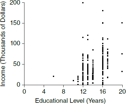
Correlation Coefficients
Two variables are positively correlated when their values tend to go up or down together, such as income and education in Figure 6. The correlation coefficient
(usually denoted by the letter r) is a single number that reflects the magnitude of a linear association and whether it is positive or negative. Figure 7 shows r for three scatter diagrams: In the first, there is no association; in the second, the association is positive and moderate; in the third, the association is positive and strong. Moving across these diagrams, the clouds of dots are increasingly clustered around a straight line that could be drawn through the cloud.
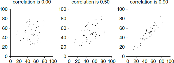
A correlation coefficient of 0 indicates no linear association between the variables. The maximum value for the coefficient is +1, indicating that all the dots fall exactly on a straight line that slopes up. Sometimes, there is a negative association between two variables: Large values of one tend to go with small values of the other. The age of a car and its fuel economy in miles per gallon illustrate the idea. Negative association is indicated by negative values for r. The extreme case is an r of –1, indicating that all the points in the scatter diagram lie on a straight line that slopes down.
Weak associations are the rule in the social sciences. In Figure 6, the correlation between income and education is about 0.4. The correlation between college grades and first-year law school grades is under 0.3 at most law schools, while the correlation between LSAT scores and first-year grades is generally about 0.4.175 The correlation between heights of fraternal twins is roughly 0.5. The correlation between heights of identical twins is about 0.9.176
175. Law School Admissions Council, Summary of 2017, 2018, and 2019 LSAT Correlation Study Results, https://perma.cc/452D-JVNP. Adjusting for range restriction boosts the median correlations to 0.44 and 0.61. Id.
176. G. Frederiek Estourgie-van Burk et al., Body Size in Five-year-old Twins: Heritability and Comparison to Singleton Standards, 9 Twin Research & Hum. Genetics 646, 649 tbl. 2 (2006), https://doi.org/10.1375/183242706778553417 (reporting correlations of about 0.59 and 0.94 for the two types of
Is the Association Linear?
The correlation coefficient has a number of limitations, to be considered in turn. The correlation coefficient is designed to measure linear association. Figure 8 shows a strong nonlinear pattern with a correlation close to zero. The correlation coefficient is of limited use with a nonlinear relationship.

Do Outliers Influence the Correlation Coefficient?
The correlation coefficient can be distorted by outliers—a few points that are far removed from the bulk of the data. The left-hand panel in Figure 9 shows that one outlier (lower right-hand corner) can reduce a perfect correlation to nearly nothing. Conversely, the right-hand panel shows that one outlier (upper right-hand corner) can raise a correlation of zero to nearly one.177 If there are extreme outliers in the data, the correlation coefficient is unlikely to be meaningful.
twins); Matthew C. Keller et al., The Genetic Correlation Between Height and IQ: Shared Genes or Assortative Mating?, 10 PLOS Genetics e1004329 tbl. 2 (2013), https://doi.org/10.1371/journal.pgen.1003451 (0.46 and 0.87); Jon Martin Sundet et al., Resolving the Genetic and Environmental Sources of the Correlation Between Height and Intelligence: A Study of Nearly 2600 Norwegian Male Twin Pairs, 8 Twin Research & Hum. Genetics 307, 309 tbl. 2 (2005), https://doi.org.10.1375/1832427054936745 (0.54 and 0.92).
177. Cf. David H. Kaye, The Dynamics of Daubert: Methodology, Conclusions, and Fit in Statistical and Econometric Studies, 87 Va. L. Rev 1933 (2001) (describing a simple linear regression in an antitrust case in which “[t]he difference between a finding by [plaintiff’s expert] of several hundred
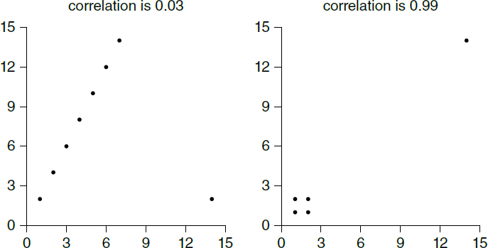
Does a Confounding Variable Influence the Coefficient?
The correlation coefficient measures the association between two variables. Researchers—and the courts—are usually more interested in causation. Causation is not the same as association. The association between two variables may be driven by a lurking variable that has been omitted from the analysis (see section titled “Is the Study Designed to Investigate Causation?” above). For an easy example, there is an association between shoe size and vocabulary among schoolchildren. However, learning more words does not cause the feet to get bigger, and larger feet do not make children more articulate. In this case, the lurking variable is easy to spot—age. In more realistic examples, the lurking variable may be harder to identify.
In statistics, lurking variables are called confounders or confounding variables. Association may reflect causation, but a large correlation coefficient is not enough to warrant causal inference. A large value of r means only that the dependent variable marches in step with the independent one: Possible reasons include causation, confounding, and coincidence. Multiple regression is one method that attempts to deal with confounders (see “Statistical Models” below).178
million dollars of damages and a finding of no damages is the inclusion in his model of a single anomalous data point”—a result that “would not be acceptable in an undergraduate econometrics class, let alone professional work” but that went undetected at trial) (quoting Brief of Amicus Curiae Dr. Daniel L. McFadden in Support of Defendants-Appellants at 15, 19, Conwood Co. v. United States Tobacco Co., 290 F.3d 768 (2002)).
178. See also Rubinfeld & Card, supra note 25. The difference between experiments and observational studies is discussed in the section titled “Descriptive Surveys and Censuses” above.
Regression Lines
The regression line can be used to describe a linear trend in the data. The regression line for income on education in the Kansas sample is shown in Figure 10. The height of the line estimates the average income for a given educational level. For example, the average income for people with 12 years of education is estimated at $35,600, indicated by the height of the line at 12 years. The average income for people with 16 years of education is estimated at $58,400.

Figure 11 shows the points for income and education that were plotted in Figure 6 with the regression line superimposed. Many straight lines could have been drawn through the data points. Some would “fit” the data better than others. The regression line in Figure 11 comes from a method known as “ordinary least squares” (OLS). Every point in the scatterplot lies some distance directly above or below the line. We can square these distances and add them up. The OLS regression line is the one line for which this sum of the squared distances is the smallest. It shows the average trend of income as education increases. Thus, the regression line indicates the extent to which a change in one variable (income) is associated with a change in another variable (education).
What Are the Slope and Intercept?
The regression line can be described in terms of its intercept and slope. Often, the slope is the more interesting statistic. In Figure 10, the slope is $5,700 per year. On average, each additional year of education is associated with an additional $5,700 of income. Next, the intercept is −$32,800. This is an estimate of
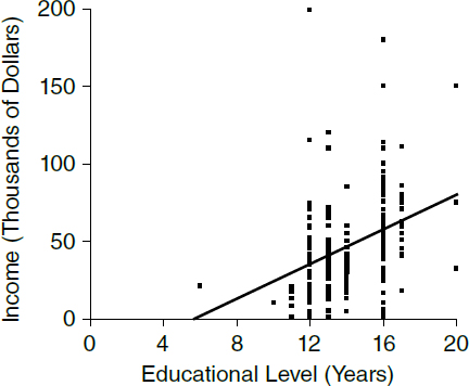
the average income for the (hypothetical) population of persons with zero years of education.179 In this case, the estimate is nonsensical (below zero!) because zero years of education is very far from the bulk of the data where income appears to grow linearly with increasing years of education.
The slope of the regression line has the same limitations as the correlation coefficient: (1) The slope may be misleading if the relationship is strongly nonlinear; and (2) the slope may be affected by confounders and outliers. With respect to (1), the slope of $5,700 per year in Figure 10 presents each additional year of education as having the same value, but some years of schooling surely are worth more and others less. With respect to (2), the association between education and income is no doubt causal, but there are other factors to consider, including family background. Compared to individuals who did not graduate from high school, people with college degrees usually come from richer and better-educated families. Thus, college graduates have advantages besides education. As statisticians
179. The regression line, like any straight line, has an equation of the form y = a + bx. Here, a is the intercept (the value of y when x = 0), and b is the slope (the change in y per unit change in x). In Figure 11, the intercept of the regression line is −$32,800 and the slope is $5,700 per year. The line estimates an average income of $58,400 for people with 16 years of education. This may be computed from the intercept and slope as follows:
−$32,800 + ($5,700 per year) × 16 years = −$32,800 + $91,200 = $58,400. The slope b is the same anywhere along the line. Mathematically, that is what distinguishes straight lines from other curves. If the association is negative, the slope will be negative too. The slope is like the grade of a road, and it is negative if the road goes downhill. The intercept is like the starting elevation of a road, and it is computed from the data so that the line goes through the center of the scatter diagram, rather than being generally too high or too low.
might say, the effects of family background are confounded with the effects of education. Statisticians often use the guarded phrases “on average” and “associated with” when talking about the slope of the regression line. This is because the slope has limited utility when it comes to making causal inferences.
What Is the Unit of Analysis?
If association between characteristics of individuals is of interest, these characteristics should be measured on individuals. Sometimes individual-level data do not exist, but rates or averages for groups are available. “Ecological” correlations are computed from such rates or averages. These correlations generally overstate the strength of an association. For example, average income and average education can be determined for men living in each state and in Washington, D.C. The correlation coefficient for these 51 pairs of averages turns out to be 0.7. However, states do not go to school and do not earn incomes. People do. The correlation for income and education for men in the United States is only 0.4. The correlation for state averages overstates the correlation for individuals—a common tendency for ecological correlations.180
Ecological analysis is often seen in cases claiming dilution in voting strength of minorities. In this type of voting rights case, plaintiffs must prove three things: (1) the minority group constitutes a majority in at least one district of a proposed plan; (2) the minority group is politically cohesive—that is, votes fairly solidly for its preferred candidate; and (3) the majority group votes sufficiently as a bloc to defeat the minority-preferred candidate.181 The first requirement is compactness; the second and third define polarized voting.
180. Correlations are computed from the March 2005 Current Population Survey for men ages 25–64. Freedman et al., supra note 14, at 149. The ecological correlation uses only the average figures, but within each state there is a lot of spread about the average. The ecological correlation smoothes away this individual variation. Cf. Gold et al., supra note 15 (suggesting that ecological studies of exposure and disease are “far from conclusive” because of the lack of data on confounding variables (a much more general problem) as well as the possible aggregation bias described here); David A. Freedman, Ecological Inference and the Ecological Fallacy, in 6 Int’l Encyclopedia of the Social and Behavioral Sciences 4027 (Neil J. Smelser & Paul B. Baltes eds., 2001).
181. See Thornburg v. Gingles, 478 U.S. 30, 50–51 (1986) (“First, the minority group must be able to demonstrate that it is sufficiently large and geographically compact to constitute a majority in a single-member district. . . . Second, the minority group must be able to show that it is politically cohesive. . . . Third, the minority must be able to demonstrate that the white majority votes sufficiently as a bloc to enable it . . . usually to defeat the minority’s preferred candidate.”). In subsequent cases, the Court has emphasized that these factors are not sufficient to make out a violation of section 2 of the Voting Rights Act. E.g., Johnson v. De Grandy, 512 U.S. 997, 1011 (1994) (“Gingles . . . clearly declined to hold [these factors] sufficient in combination, either in the sense that a court’s examination of relevant circumstances was complete once the three factors were found to exist, or in the sense that the three in combination necessarily and in all circumstances
The secrecy of the ballot box means that polarized voting cannot be directly observed. Instead, plaintiffs in voting rights cases rely on ecological regression, with scatter diagrams, correlations, and regression lines to estimate voting behavior by groups and demonstrate polarization.182 The unit of analysis typically is the precinct. For each precinct, public records can be used to determine the percentage of registrants in each demographic group of interest, as well as the percentage of the total vote for each candidate—by voters from all demographic groups combined. Plaintiffs’ burden is to determine the vote by each demographic group separately.
Figure 12 shows how the argument unfolds. Each point in the scatter diagram represents data for one precinct in the 1982 Democratic primary election for auditor in Lee County, South Carolina. The horizontal axis shows the percentage of registrants who are white. The vertical axis shows the turnout rate for the white candidate. The regression line is plotted too. The slope would be interpreted as the expected increase in the proportion supporting the white candidate for each 1% increase in the proportion of white registrants in the precinct. The intercept then would be the expected support for the white candidate in a precinct with no white registrants (an all-Black precinct).183 The validity of such estimates is contested in the statistical and legal literature.184
demonstrated dilution.”). On the legal framework and its problems, see Christopher S. Elmendorf et al., Racially Polarized Voting, 83 U. Chi. L. Rev. 587 (2016); D. James Greiner, Re-Solidifying Racial Bloc Voting: Empirics and Legal Doctrine in the Melting Pot, 86 Ind. L.J. 447 (2011); Nicholas O. Stephanopoulos, The Relegation of Polarization, 83 U. Chi. L. Rev. Online 160, 168 (2017).
182. Less readily visualized procedures also are used. See, e.g., Ecological Inference: New Methodological Strategies (Gary King et al. eds., 2004); Loren Collingwood et al., The R Journal: eiCompare: Comparing Ecological Inference Estimates Across EI and EI:R×C, R J., Dec. 2016, at 92, https://perma.cc/U5JH-GBEM. We confine our explanation to the simplest (bivariate linear) form of ecological regression. All the methods confront the same fundamental problem of inferring associations at the level of individuals from differences among groups that include heterogeneous subgroups of individuals. Given this common issue and objective, one might think that the phrase “ecological inference” would be a broad umbrella term, but especially in voting rights litigation, the phrase usually refers to one particular procedure that is more complex than traditional bivariate ecological regression. See, e.g., Luna v. County of Kern, 291 F. Supp. 3d 1088, 1118 (E.D. Cal. 2018) (describing differences between ecological regression (ER) and “[e]cological inference (‘EI’), developed by political scientist Gary King in 1997 [that] is ‘similar to, but largely regarded as an improvement upon’ the ER methodology endorsed in Gingles”). But see Elmendorf & Spencer, supra note 172, at 2180 (referring to “statistically tenuous techniques of ecological inference”); Greiner, supra note 181, at 449 (observing that “analyzing census data (usually) and precinct-level vote returns via a set of methods collectively called ‘ecological inference’ has been a staple since the mid 1980s”).
183. By definition, the turnout rate equals the number of votes for the candidate, divided by the number of registrants; the rate is computed separately for each precinct. The intercept of the line in Figure 11 is 4%, and the slope is 0.52. Plaintiffs would conclude that only 4% of the voters in an all-Black precinct would be expected to vote for the white candidate, while 4% + 52% = 56% of the voters in an all-white precinct would be expected to vote for the white candidate, which demonstrates polarization.
184. E.g., Moon Duchin & Douglas M. Spencer, Models, Race, and the Law, 130 Yale L.J. Forum 744 (2021); Elmendorf & Spencer, supra note 172, at 2203 (“Ecological inference as

Statistical Models
Statistical models are widely used in the social sciences and in litigation. For example, the census suffers an undercount, more severe in certain places than others.
traditionally practiced relies on heroic assumptions, elides questions about statistical precision, and uses post-hoc corrections to paper over mathematically impossible results. . . .”) (note omitted). For references to some of the statistical literature, see Collingwood et al., supra note 182, at 92–94. The use of ecological regression and other quantitative methods increased considerably after the Supreme Court noted in Thornburg v. Gingles, 478 U.S. 30, 53 n.20 (1986), that “[t]he District Court found both methods [extreme case analysis and bivariate ecological regression analysis] standard in the literature for the analysis of racially polarized voting.” See Bruce M. Clarke & Robert Timothy Reagan, Federal Judicial Center, Redistricting Litigation: An Overview of Legal, Statistical, and Case-Management Issues (2002); D. James Greiner, The Quantitative Empirics of Redistricting Litigation: Knowledge, Threats to Knowledge, and the Need for Less Districting, 29 Yale L. & Policy Rev. 527 (2011); D. James Greiner, Ecological Inference in Voting Rights Act Disputes: Where Are We Now, and Where Do We Want to Be?, 47 Jurimetrics J. 115, 117, 121 (2007).
Redistricting plans based predominantly on racial considerations are unconstitutional unless narrowly tailored to meet a compelling state interest. Shaw v. Reno, 509 U.S. 630 (1993). Whether compliance with the Voting Rights Act can be considered a compelling interest is an open question, but efforts to sustain racially motivated redistricting on this basis have not fared well before the Supreme Court. See Abrams v. Johnson, 521 U.S. 74 (1997); Shaw v. Hunt, 517 U.S. 899 (1996); Bush v. Vera, 517 U.S. 952 (1996); Abbott v. Perez, 585 U.S. 579 (2018); but see Alabama Legislative Black Caucus v. Alabama, 575 U.S. 254 (2015); Bethune-Hill v. Virginia State Bd. of Elections, 580 U.S. 178 (2017); Cooper v. Harris, 581 U.S. 285 (2017).
185. Data from James W. Loewen & Bernard Grofman, Recent Developments in Methods Used in Vote Dilution Litigation, 21 Urb. Law. 589, 591 tbl.1 (1989).
If some statistical models are to be believed, the undercount can be corrected—moving seats in Congress and millions of dollars a year in tax5185 funds.186 Other models purport to lift the veil of secrecy from the ballot box, enabling the experts to determine how minority groups have voted—a crucial step in voting rights litigation (see section titled “Regression Lines” above). This section discusses the statistical logic of regression models.
A regression model attempts to combine the values of certain variables (the independent variables) to get expected values for another variable (the dependent variable). The model can be expressed in the form of a regression equation. A simple regression equation has only one independent variable; a multiple regression equation has several independent variables. Coefficients in the equation will be interpreted as showing the effects of changing the corresponding variables. This is justified in some situations, as the next example demonstrates.
Hooke’s law (named after Robert Hooke, England, 1653–1703) describes how a spring stretches in response to a load: Strain is proportional to stress. To verify Hooke’s law experimentally, a physicist will make a number of observations on a spring. For each observation, the physicist hangs a weight on the spring and measures its length. A statistician could develop a regression model for these data:
| length= a + (b× weight) + ε | (1) |
The error term, denoted by the Greek letter ε (epsilon) is needed because measured length will not be exactly equal to a + (b× weight). If nothing else, error in measuring the spring’s length must be reckoned with.187 The model takes ε as “random error”—behaving like draws made at random with replacement from a box of tickets. Each ticket shows a potential error, which will be realized if that ticket is drawn. The average of the potential errors in the box is assumed to be zero.188
Equation (1) has two parameters, a and b. These constants of nature characterize the behavior of the spring: a is length under no load, and b is elasticity (the increase in length per unit increase in weight). By way of numerical illustration, suppose a is 400 and b is 0.05. If the weight is 1, the length of the spring is expected to be
400 + (0.05 × 1) = 400.05.
186. See Brown et al., supra note 36.
187. We will assume that the physicist uses a perfectly accurate and unchanging set of standard weights.
188. In standard statistical terminology, the process of measuring length here is unbiased.
If the weight is 3, the expected length is
400 + (0.05 × 3) = 400 + 0.15 = 400.15.
In either case, the actual length will differ from expected, by a random error ε.
In the simplest situation, the ε’s for different observations on the spring are assumed to be independent and identically distributed, with a mean of zero. “Independent” means that, for any two observations using the same weight, the chances for one ε do not depend on outcomes for the other. If the errors are like draws made at random with replacement from a box of tickets, as we assumed earlier, they are independent—the box will not change from one draw to the next. “Identically distributed” means that the chance behavior of the two ε’s is the same: They are drawn at random from the same box.
The parameters a and b in equation (1) are not directly observable, but they can be estimated by the method of least squares.189 Statisticians often denote estimates by hats. Thus, is the estimate for a, and is the estimate for b. The values of and are chosen to minimize the sum of the squared prediction errors. These errors are also called residuals. They measure the difference between the actual length of the spring and the predicted length, the latter being + × weight:
| actual length = + ( × weight) + residual | (2) |
Of course, no one really imagines there to be a box of tickets hidden in the spring. However, the variability of physical measurements (under many but by no means all circumstances) does seem to be remarkably like the variability in draws from a box.190 In short, the statistical model corresponds rather closely to the empirical phenomenon.
Equation (1) is a statistical model for the data, with unknown parameters a and b. The error term ε is not observable. The model is a theory—and a good one—about how the data are generated. By contrast, equation (2) is a regression equation that is fitted to the data: The intercept , the slope , and the residual can all be computed from the data. The results are useful because is a good estimate for a, and is a good estimate for b. (Similarly, the residual is a good approximation
189. See section titled “Regression Lines” above. It might seem that a is observable; after all, we can measure the length of the spring with no load. However, the measurement is subject to error, so we observe not a, but a + ε. See equation (1). The parameters a and b can be estimated, even estimated very well, but they cannot be observed directly. The least squares estimates of a and b are the intercept and slope of the regression line. See section titled “What Are the Slope and Intercept?” above and Freedman et al., supra note 14, at 208–10. The method of least squares was developed by Adrien-Marie Legendre (France, 1752–1833) and Carl Friedrich Gauss (Germany, 1777–1855) to fit astronomical orbits.
190. This is the Gauss model for measurement error. See Freedman et al., supra note 14, at 450–52.
to ε.) Without the theory, these estimates would be less useful. Is there a theoretical model behind the data processing? Is the model justifiable? These questions can be critical when it comes to making statistical inferences from the data.
These points apply to more complicated statistical models. The simple linear regression model exemplified in equation (1) can be extended in many ways. If another variable might contribute to or be associated with a response, an additional term (constant× variable) can be added to the right-hand side of the equation. Furthermore, the relationship between the independent and dependent variables need not be linear. For instance, to model measurements of the distance d a ball dropped from the Leaning Tower of Pisa falls in a few seconds, Newton’s laws imply that we should use a model with the time variable squared.191 Also, variables that are dichotomous rather than continuous (such as whether a mouse will develop cancer after exposure to a food additive) can be part of a regression model.192
In social science and legal applications, such advanced statistical models often are invoked—even when they lack an independent theoretical basis. Hooke’s law—incorporated in equation (1)—is relatively easy to test experimentally. For something like the salaries that an employer pays to workers, validation of a proposed relationship between the dependent variable and the independent ones would be difficult to validate experimentally. When expert testimony relies on statistical models, the court may well inquire, what are the assumptions behind the model, and why do they apply to the case at hand? The assumptions being questioned can include the choice of variables in the regression and the nature of the assumed relationship. It is important to distinguish between two situations:
- The nature of the relationship between the variables is known and regression is being used to make quantitative estimates of parameters in that relationship, and
- The nature of the relationship is largely unknown and regression is being used to determine the nature of the relationship—or indeed whether any relationship exists at all.
Regression was developed to handle situations of the first type, with Hooke’s law being an example. The basis for the second type of application is analogical, and the tightness of the analogy is an issue worth exploration.193
191. The model would be distance = a + (b × seconds2) + ε instead of distance = a + (b × seconds) + ε.
192. Such extensions and modifications of simple linear regression are introduced in the Reference Guide on Multiple Regression and Advanced Statistical Models; see also Andrew Gelman et al., Regression and Other Stories (2020).
193. See, e.g., David A. Freedman, Statistical Models and Causal Inference: A Dialogue with the Social Sciences (David Collier et al. eds., 2009); Andrew Gelman, Review Essay: Causality and Statistical Learning, 117 Am. J. Sociology 955 (2011).
For most questions of legal interest, a wide variety of models can be used. This is only to be expected, because the science does not dictate specific equations and causal relationships. In a strongly contested case, each side will have its own model (series of models), presented by its own expert. The experts often reach opposite conclusions. The dialogue might continue with an exchange about which models produce admissible results, or more convincing ones. Although assumptions about the form of the model or the error component are challenged in court from time to time, arguments more commonly revolve around the choice of variables. One model may be questioned because it omits variables that arguably should be included—for example, skill levels or prior evaluations in an employment discrimination case.194 Another model may be challenged because it includes tainted variables reflecting past discriminatory behavior by the firm.195 One expert may emphasize how remarkably well the fitted regression curve or surface fits; another expert may reply that the model, especially a complicated one, is ad hoc—it is tailored to the data in question and cannot be relied on to work well with other data arising from the same data-generating process.196 The court or jury must decide which model—if any—fits the occasion.197
The frequency with which regression models are used is no guarantee that they are the best choice for any particular problem.198 Indeed, from one perspective, a regression or other statistical model may seem to be a marvel of mathematical rigor. From another perspective, the model could be a set of assumptions,
194. E.g., Bazemore v. Friday, 478 U.S. 385 (1986); In re Linerboard Antitrust Litig., 497 F. Supp. 2d 666 (E.D. Pa. 2007).
195. E.g., McLaurin v. Nat’l R.R. Passenger Corp., 311 F. Supp. 2d 61, 65–66 (D.D.C. 2004) (holding that the inclusion of two allegedly tainted variables was reasonable in light of an earlier consent decree); see also In re Urethane Antitrust Litig., 166 F. Supp. 3d 501, 506 (D.N.J. 2016) (“courts have declined to fault a regression model for excluding variables that could have been manipulated by a defendant in furtherance of an antitrust conspiracy”).
196. E.g., Students for Fair Admissions, Inc. v. Univ. of N.C., 567 F. Supp. 3d 580, 622 (M.D.N.C. 2021) (“both experts agree that the degree of overfit is a factor they must take into account, the parties disagree on how to measure it”), rev’d, 600 U.S. 181 (2023); In re Urethane Antitrust Litig., 166 F. Supp. 3d at 505 (predictions were admissible despite the argument “that the models in this case were able to accurately match prices during the benchmark period not because they are reliable, but because they are ‘overfit’”).
197. E.g., Chang v. Univ. of R.I., 606 F. Supp. 1161, 1207 (D.R.I. 1985) (“it is plain to the court that [defendant’s] model comprises a better, more useful, more reliable tool than [plaintiff’s] counterpart”); Presseisen v. Swarthmore Coll., 442 F. Supp. 593, 619 (E.D. Pa. 1977) (“[E]ach side has done a superior job in challenging the other’s regression analysis, but only a mediocre job in supporting their own . . . and the Court is . . . left with nothing.”), aff’d, 582 F.2d 1275 (3d Cir. 1978).
198. See, e.g., In re Urethane Antitrust Litig., 166 F. Supp. 3d at 504–05 (although “there are an abundance of judicial decisions supporting the premise that regression models can be a reliable tool for measuring damages in an antitrust case,” plaintiff’s “regression models must stand on their own two feet”).
supported only by the say-so of the testifying expert. Intermediate judgments are also possible.199
Data Science and Statistical Machine Learning
“Statistical science” has been described as “the discipline of learning about the world from data,”200 and “statistics” as the art of “learning from data.”201 Yet, there are now journals,202 university degree programs,203 and job positions204 dedicated—not to statistics—but to “data science.” Spurred by the availability of large and heterogeneous data collections, computer-intensive algorithmic procedures for making predictions and classifications are increasingly applied in science, business, and law enforcement.205 These procedures have often been termed “analytics,” “artificial intelligence,” and “machine learning.” How might testimony and reports from “data scientists” differ from more traditional data analyses of statisticians? What statistical considerations or methods should be used to validate the output from machine learning approaches? To supply background information for approaching these questions, this section describes the
199. See, e.g., David W. Peterson, Reference Guide on Multiple Regression, 36 Jurimetrics J. 213, 214–15 (1996) (review essay); see supra note 25 for references to a range of academic opinion. More recently, some investigators have turned to graphical models. However, these models have serious weaknesses of their own. See, e.g., David A. Freedman, Graphical Models for Causation, and the Identification Problem, 28 Evaluation Rev. 267 (2004), https://doi.org/10.1177/0193841X04266432.
200. Spiegelhalter, supra note 95, at 404 (Basic Books edition).
201. This is the subtitle of the Penguin Books edition of Speigelhalter, supra note 95.
202. The Harvard Data Science Review (https://perma.cc/T87V-VEP3), for example, “aim[s] to publish content that help define and shape data science as a scientifically rigorous and globally impactful multidisciplinary field based on the principled and purposed production, processing, parsing, and analysis of data.”
203. U.S. News & World Rep., Best Undergraduate Data Science Programs, https://www.usnews.com/best-colleges/rankings/computer-science/data-analytics-science.
204. The Bureau of Labor Statistics has an occupational category for “data scientists” that excludes statisticians. U.S. Bureau of Labor Statistics, Occupational Employment and Wages, May 2021, https://www.bls.gov/oes/current/oes152051.htm.
205. Applications of particular legal interest include predicting criminal behavior at the individual level (see, e.g., Richard A. Berk & J. Bleich, Statistical Procedures for Forecasting Criminal Behavior: A Comparative Assessment, 12 Criminology & Public Policy 513 (2013), https://doi.org/10.1111/1745-9133.12407, classifying trace evidence such as toolmarks according to their source (see, e.g., ANSI/ASB 062, Standard for Topography Comparison Software for Toolmark Analysis (2021)), and forensic speaker recognition (see, e.g., Geoffrey Stewart Morrison & William C. Thompson, Assessing the Admissibility of a New Generation of Forensic Voice Comparison Testimony, 18 Colum. Sci. & Tech. L. Rev. 326, 345–46 (2017); Zhongxin Bai & Xiao-Lei Zhang, Speaker Recognition Based on Deep Learning: An Overview, 140 Neural Networks 65 (2021), https://doi.org/10.1016/j.neunet.2021.03.004.
general nature of “data science” and sketches the broad outlines of the statistical thinking that is crucial to evaluating results from machine learning.206
What Is Data Science?
“There is a wide variety of definitions and criteria for what constitutes data science,” making the term something of “a buzzword.”207 Typical definitions, such as “a collection of techniques used to extract value from data [that] rely on finding useful patterns, connections, and relationships within data,”208 do not distinguish data science from applied statistics.209 For centuries, statisticians have been concerned with discerning patterns and regularities in natural and social processes and with predicting uncertain outcomes.
Nonetheless, data science has emerged as a combination of statistics, computing, and informatics ideas about the collection, storage, analysis, visualization, and reporting of data. Advances in technology, computing, and data-storage capacity have produced a data explosion in commerce (partly driven by online shopping), science (massive sky surveys, environmental and climate data, genomic information, and much more), and digitalized voice, text, and pictures collected to support speech and image recognition.210 The “data science” that “extracts value” from these new troves of data is a conglomeration of mathematically grounded modeling methods from traditional statistics and highly pragmatic procedures for making predictions and classifications. The latter methods often fall under the rubric of “machine learning” and are sketched in the next section.
What Is Machine Learning?
“Machine learning” refers to methods for using data to classify objects or patterns into categories, and to produce predictions of future outcomes or events. The
206. For a general discussion of AI and related societal implications, see James E. Baker & Laurie N. Hobert, Reference Guide on Artificial Intelligence, in this manual.
207. Vijay Kotu & Bala Deshpande, Data Science: Concepts and Practice 1 (2d ed. 2019).
208. Id.; see also Bradley Efron & Trevor Hastie, Computer Age Statistical Inference: Algorithms, Evidence, and Data Science 451 (2016) (noting that “[t]he data science association defines a practitioner as one who ‘uses scientific methods to liberate and create meaning from raw data’”).
209. See Matthew A. Jay & Mario Cortina Borja, Quomoto Dicitur “Data Science” Latine, Significance, Aug. 2020, at 26.
210. Initially the increased amount of data was heralded as the dawn of a Big Data era involving Big Data specialists. See Francis X. Diebold, What’s the Big Idea? “Big Data” and Its Origins, Significance, Feb. 2021, at 36–37. “Big” can refer to the number of units (people, social media posts, galaxies, etc.) in a dataset (“examples” in a database). It also can refer to the number of variables for each unit (the “features” of the examples). Genomes are big—they have billions of base pairs—even if they come from only a handful of people.
equations or procedures rely on computers. Of course, classification and prediction are tasks that humans do, either intuitively or with experience and expert training. Thus, machine learning (ML) is a subfield of “artificial intelligence” (AI), which seeks to build machines that perform tasks we associate with intelligent agents.211
ML is closely related to statistics. Some methods that are packaged as ML or AI are nothing fundamentally new.212 For example, regression models can play a role. An easily understood example—predicting the first-year grade-point average (GPA) of a student entering law school from only one variable—illustrates some of the terminology. The school knows the LSAT score and the subsequent first-year GPA of every student in last year’s class. It can make predictions by fitting a straight line to those data points. As explained in the sections titled “Correlation and Regression” and “What Inferences Can Be Drawn from the Data?” above, the fitted line could have the mathematical form GPA = + × LSAT, where and are the line’s intercept and slope as estimated from the data.213 The estimates could come from equations for the values that minimize the sum of the squared differences between each data point and the fitted line. (That criterion, in turn, can be justified by a regression model in which GPA= a + b× LSAT+ ε, where a and b are the unknown parameters and ε is a normally distributed error term.) With the fitted equation in place (and under the assumption that the relationship between the variables for last year’s students will continue to apply), the prediction of an applicant’s
211. AI is extremely broad in its scope and tools, with no single, commonly accepted definition. See, e.g., Stuart J. Russell & Peter Norvig, Artificial Intelligence: A Modern Approach (3d ed. 2010). Indeed, “so far at least, all the candidates [for a definition] have substantial flaws.” Richard A. Berk, Artificial Intelligence, Predictive Policing, and Risk Assessment for Law Enforcement, 4 Ann. Rev. Criminology 209, 211 (2021). For a time, AI focused on building symbolic representations of the world and developing rule- or case-based systems that could reason based on those representations. See, e.g., Philip Leith, The Rise and Fall of the Legal Expert System, 1 European J. L. & Tech. No. 1 (2010), https://perma.cc/E8MF-JTFU. Although statisticians and machine-learning researchers do not think of their work as necessarily being motivated by traditional AI goals such as elucidating how the brain processes information, the statistical and algorithmic methods have produced automated systems that work well for narrow tasks. These accomplishments are now designated “narrow” or “weak” AI. However, “the artificial intelligence of today is computer code written to accomplish a specific empirical task. Restated, it is just a computational procedure. In law enforcement settings, these procedures are by and large enhancements of activities that humans are already performing. Arguably, computers can do them faster and more accurately, but the internal operations are far removed from the way humans actually think. It is not even clear that the term intelligence applies.” Berk, supra, at 212.
212. Susan Athey & Guido W. Imbens, Machine Learning Methods that Economists Should Know About, 11 Ann. Rev. Econ. 685, 689 (2019), https://doi.org/10.1146/annrev-economics-080217-053433 (observing that “[o]ne source of confusion is the use of new terminology in ML for concepts that have well-established labels in the older literatures” and providing examples in the context of regression analysis); Berk, supra note 211, at 223–24 (some crime-forecasting procedures presented as ML “are a rebranding of statistical tools developed more than 50 years ago”).
213. Additional predictors and other functional forms could be explored with the statistical procedures mentioned in the Reference Guide on Multiple Regression and Advanced Statistical Models.
score is simple arithmetic—one multiplication and one addition. The calculations, including the estimates of a and b, could be done by hand for a single law school, or the LSAT–GPA data could be entered into a spreadsheet or a statistical package of software that would generate the prediction equation and any desired prediction based on it. Next year, the machine will have new “training” data (another set of actual GPAs and LSATs) from which it can “learn” to make predictions (from a regression equation with updated, estimated values for the parameters a and b).
Prediction by simple linear regression is so well established it is unlikely to be packaged as machine learning. That phrase is more likely to be encountered with procedures that depart from such explicit modeling and that are said to be “algorithmic.”214 The word itself is not very revealing. Algorithms are step-by-step instructions for computing something. They can be written down in English or another natural language, or depicted in a flow chart. Then they can be implemented on a computer after they are converted into a specific computer programming language (“code”).
The regression model-based procedure for predicting GPA entails two parts that can be called algorithmic. First, there was an algorithm for finding the particular regression line.215 Second, this line enables us to write down an algorithm for calculating the predicted value. This second algorithm might go as follows: (1) input the applicant’s LSAT score; (2) multiply it by the value found from all the data; add the value found for to the result; (3) output the result of step (2) for the predicted GPA.
Because algorithms underlie all computation, it is not the existence of algorithms that makes ML distinctive. It is the willingness to develop algorithms for predictions or classifications without necessarily positing a statistical model of how the data arise. Statisticians historically relied on statistical models with a relatively small number of interpretable parameters (like the intercept a and the slope b of the simple regression line) and used manageably small datasets to estimate the values of these parameters. But models with many parameters are characteristic of ML.216
To convey the rough idea, let’s imagine that instead of imposing the linear regression model on the LSAT–GPA data, we used the following algorithm: (1) compute the average GPA for the students with LSATs ranging from 120–130,
214. E.g., Berk, supra note 211, at 12 (“An essential feature of artificial narrow intelligence is that it depends on algorithms, not models.”); Moritz Hardt & Benjamin Recht, Patterns, Predictions, and Actions: Foundations of Machine Learning 11 (2020) (“Machine learning is to a large extent the study of algorithmic prediction.”); Efron & Hastie, supra note 208, at 451 (“the emphasis is on the algorithmic processing of large data sets for the extraction of useful information, with the prediction algorithms as exemplars”).
215. The equations for estimating a and b in the regression model are solved by a particular series of additions, subtractions, and multiplications that are guaranteed to give the specific values and that minimize the sum of the squared deviations between each data point and the overall fitted line.
216. For discussion of how such procedures relate to more traditional statistical methods, see Special Issue: Commentaries on Breimen’s Two Cultures Paper, 7 Observational Stud. 1–234 (2021).
130–140, and so on through 170–180; (2) plot these averages as heights at the midpoints of the intervals (125, 135, . . . , 175); (3) connect them to form a jagged line, and (4) use this jagged line to make predictions. Of course, one might ask why widths of 10 LSAT points should be used. Why not use shorter or longer segments for computing the means? An optimization procedure that reserves some of the data to try out different possibilities could help identify which width to use.217 The approach resembles engineering by trial and error.218
Our jagged line would not be used in practice. There are better procedures for fitting a curve to a cloud of data points. The slice-compute-and-connect algorithm is here only to illustrate the idea of a highly data-driven procedure that leads to an algorithm (corresponding to the resulting jagged line) for making the predictions. The jagged line would hug the data more tightly than the single regression line with only two parameters. Maybe it would produce better predictions.
A number of important ML procedures do not yield any explicit equation (like the single regression line or the more complex jagged line) for making predictions or classifications. The two stages are done together, and the relevant variables are not necessarily pre-defined by the developer of the prediction model. Also, the features of the data that have the most influence on the output often are unknown.
What Statistical Questions Arise with Machine Learning Studies?
Although machine-learning advocates sometimes advertise that their methods make very few assumptions and provide great flexibility, they are still subject to the statistical and logical issues discussed in previous sections. Data quality,
217. We could reserve a random 10% of the data and develop the jagged line on the remaining 90% using a width of, say, two LSAT points. Then we check how well the fitted line works on the reserved 10% by finding the correlation between the fitted line’s predictions and the reserved data points. We do this repeatedly, say 10 times, to get an average correlation for the jagged line with the two-point width. Then we return to the full training set and repeat this 10-fold train-test process for other values of the width. Finally, we pick the width with the highest correlation (“cross-validity”) and apply it to the full training set (100% of the data). That gives the prediction line.
218. Moritz Hardt & Benjamin Recht, Patterns, Predictions, and Actions: Foundations of Machine Learning 146 (2020) (“Methodologically, much of modern machine learning practice rests on a variant of trial and error, which we call the train-test paradigm. Practitioners repeatedly build models using any number of heuristics and test their performance to see what works. Anything goes as far as training is concerned, subject only to computational constraints, so long as the performance looks good in testing.”).
robustness, and transparency are a few of the issues that can arise.219 We consider these three in turn.220
Is the Dataset Appropriate and of Sufficient Quality?
To begin with, as with traditional statistical methods, care is needed in the assembly of the data used to build and test the algorithms. Algorithms must be developed on data that are accurate and representative of the type of data to which they will be applied. For example, a study on diagnosing autism using ML excluded the data corresponding to borderline cases of autism. That made the test set unrepresentative of the general population; moreover, when a dataset that included the difficult-to-diagnose cases was used, the accuracy declined.221
Is the Predictor or Classifier Robust?
Second, robustness is also a vital issue. The goal of ML is not merely to find some complex pattern in the data; it is to discover generalizable patterns. For instance, a complex equation using many characteristics of each student to predict law school GPA could fit last year’s data splendidly, but it might be idiosyncratic to the “training” data. In other words, it might not generalize to next year’s data. This is known as overfitting. It can occur with traditional statistical techniques but is a greater risk with the high-dimensional (many variables) algorithmic approaches
219. For reviews of ML studies identifying frequent mistakes or departures from good practice, see Sayash Kapoor & Arvind Narayanan, Leakage and the Reproducibility Crisis in Machine-learning-based Science, 4 Patterns 100804 (2023), https://doi.org/10.1016/j.patter.2023.100804; Michael Roberts et al., Common Pitfalls and Recommendations for Using Machine Learning to Detect and Prognosticate for COVID-19 Using Chest Radiographs and CT Scans, 3 Nature Machine Intelligence 199 (2021); Laure Wynants et al., Prediction Models for Diagnosis and Prognosis of Covid-19: Systematic Review and Critical Appraisal, 369 Brit. Med. J. m1328 (2020), https://doi.org/10.1136/bmj.m1328. The extent to which published studies using ML-methods produce results that are superior to more traditional statistical methods is an active area of research. See, e.g., Mohammad Ziaul Islam Chowdhury et al., Prediction of Hypertension Using Traditional Regression and Machine Learning Models: A Systematic Review and Meta-Analysis, 17 PLoS ONE e0266334 (2022), https://doi.org/10.1371/journal.pone.0266334; Xuan Song et al., Comparison of Machine Learning and Logistic Regression Models in Predicting Acute Kidney Injury: A Systematic Review and Meta-Analysis, 151 Int’l J. Med. Informatics 104484 (2021), https://doi.org/10.1016/j.ijmedinf.2021.104484.
220. The choice of statistics to indicate the accuracy of a predictor or classifier is another important topic.
221. Daniel Bone et al., Applying Machine Learning to Facilitate Autism Diagnostics: Pitfalls and Promises, 45 J. Autism & Developmental Disorders 1121 (2015), https://doi.org/10.1007/s10803-014-2268-6.
that characterize modern machine learning. “Internal validation” can be achieved by holding out some data in the training set as the algorithm is developed and measuring how well the algorithm predicts or classifies those test data.222 But such internal validation is not sufficient. “External validation” requires testing the algorithm on data from a different source, and results from those tests should be reported. Furthermore, even if external validation has been performed at one point in time, confidence in continued predictive accuracy requires ongoing efforts to ensure that the relationships among variables in the data are not changing over time (or to revise the equations or algorithms if they are).
Is the Predictor or Classifier Too Opaque?
Finally, ML algorithms can be difficult to interpret, especially when the patterns that are “learned” may not be represented in easily decoded forms. This can make it hard to tell when the data environment is changing in ways that will lead to poorer performance. It also can mask the fact that the algorithm has access to features that should not be part of the data. For example, when researchers rushed to apply ML methods to COVID-19 diagnosis from chest X-rays and CT scans, many of them unwittingly used a dataset that contained chest scans of children who did not have COVID as their examples of what non-COVID cases looked like. As a result, the ML diagnoses were relying on features identifying children rather than COVID.223 Concerns such as these are prompting the development of methods for gaining insight into how opaque ML systems are functioning224 and to lists of criteria for judging when ML algorithms are most likely to be trustworthy.225
222. This is a very rough description of cross-validation with data available when developing the algorithm. For discussion of data-splitting and resampling techniques, see, for example, Max Kuhn & Kjell Johnson, Applied Predictive Modeling 61–92 (2013).
223. Id.
224. Berk, supra note 211, at 231.
225. E.g., Kapoor & Narayanan, supra note 219; Russell A. Poldrack et al., Establishment of Best Practices for Evidence for Prediction: A Review, 77 JAMA Psychiatry 534 (2020), https://doi.org/10.1001/jamapsychiatry.2019.3671; Roberts et al., supra note 219.
Appendix: Conditional Probability and Bayes’ Rule
What Do Probabilities Apply To?
The mathematical theory of probability consists of theorems derived from axioms and definitions. Mathematical reasoning is seldom controversial, but there may be disagreement as to how the theory should be applied. For example, statisticians may differ on the interpretation of data in specific applications. Moreover, there are two main schools of thought about the foundations of statistics: frequentist and Bayesian (also called objectivist and subjectivist).226
Frequentists see probabilities as empirical facts. When a fair coin is tossed, the probability of heads is taken to be 1/2; this value is justified by the argument that if the experiment is repeated a large number of times, the coin will land heads about one-half the time. If a fair die is rolled, the probability of getting an ace (one spot) is 1/6. If the die is rolled many times, an ace will turn up about one-sixth of the time.227 Generally, if a chance experiment can be repeated, the relative frequency of an event approaches (in the long run) its probability. By contrast, a Bayesian considers probabilities as representing not facts but degrees of belief: in whole or in part, probabilities are subjective.228
226. The extent to which statisticians using Bayesian methods are overtly subjective in their analyses varies. “Objective Bayesians” use Bayes’ rule without eliciting prior probabilities from subjective beliefs. One strategy is to use preliminary data to estimate the prior probabilities and then apply Bayes’ rule to that empirical distribution. This “empirical Bayes” procedure avoids the charge of subjectivism at the cost of departing from a fully Bayesian framework. With ample data, it can be effective, and the estimates or inferences can be understood in frequentist terms. Another “objective” approach is to use “noninformative” priors that are supposed to be independent of all data and prior beliefs. However, the choice of such priors can be questioned, and the approach has been contested by frequentists and subjective Bayesians. E.g., Joseph B. Kadane, Is “Objective Bayesian Analysis” Objective, Bayesian, or Wise?, 1 Bayesian Analysis 433 (2006), https://perma.cc/CSN9-35G5; Jon Williamson, Philosophies of Probability, in Philosophy of Mathematics 493 (Andrew Irvine ed., 2009) (discussing the challenges to objective Bayesianism).
227. Probabilities may be estimated from relative frequencies, but probability itself is a subtler idea. For example, suppose a computer prints out a sequence of ten letters H and T (for heads and tails), which alternate between the two possibilities H and T as follows: H T H T H T H T H T. The relative frequency of heads is 5/10 or 50%, but it is not at all obvious that the chance of an H at the next position is 50%. There are difficulties in both the subjectivist and objectivist positions. See Freedman, supra note 167.
228. “Subjective” is not necessarily the same as arbitrary. The degrees of belief must obey the same mathematical rules (axioms and theorems) as relative frequencies do, and the personal choices for particular numbers can be subjected to interpersonal standards for acceptance by other individuals.
What Are Conditional Probabilities?
Conditional probability is the probability of one event given that another has occurred. For example, suppose a fair coin is tossed twice. One event is that the coin will land heads up both times (HH). Another event is that at least one H will be seen. Before the coin is tossed, there are four possible, equally likely, outcomes: HH, HT, TH, TT. So the probability of HH is 1/4. However, if we know that at least one head has been obtained, then we can rule out two tails TT. In other words, given that at least one H has been obtained, the conditional probability of TT is 0, and the first three outcomes have conditional probability 1/3 each. In particular, the conditional probability of HH is 1/3. This is usually written as P(HH|at least one H) = 1/3. More generally, the probability of an event C is denoted P(C); the conditional probability of D given C is written as P(D|C).
Two events C and D are independent if the conditional probability of D given that C occurs is equal to the conditional probability of D given that C does not occur. Using ~C to denote the event that C does not occur, C and D are independent if P(D|C) = P(D|~C). If C and D are independent, then the probability that both occur is equal to the product of the probabilities:
| P(C and D) = P(C) × P(D) | (3) |
This is the multiplication rule (or product rule) for independent events. If events are dependent, then conditional probabilities must be used:
| P(C and D) = P(C) × P(D|C) | (4) |
This is the multiplication rule for dependent events. Statisticians caution against, but sometimes succumb to, using the multiplication rule for independent events when the events are dependent.229
What Is Bayes’ Rule?
If we use probabilities to describe uncertainty regarding hypotheses as well as to describe events, we can use the formulas for conditional probabilities to obtain an equation known as Bayes’ rule that has been proposed to guide legal factfinding. If
229. E.g., William Kruskal, Miracles and Statistics: The Casual Assumption of Independence, 83 J. Am. Stat. Ass’n 929 (1988), https://doi.org/10.2307/2290117. A famous case of multiplication without apparent attention to dependence is People v. Collins, 438 P.2d 33 (Cal. 1968). For more examples, see infra note 238.
two mutually exclusive hypotheses H0 and H1 describe all the ways that an event A could occur,230 it is easy to show that231
| (5) |
This is one way of expressing Bayes’ rule. It yields the conditional probability of hypothesis H1 given that event A has occurred.
For a stylized example in a criminal case, suppose that blood from a single source is found at the scene of a crime and that the defendant in the case has type A blood. It is natural to have one hypothesis H0 propose that the blood came from a person other than the defendant; the other hypothesis H1 is that the blood came from the defendant; the event A is the event that blood from the crime scene is found to be type A. Then P(H0) is the “prior probability” of H0, based on subjective judgment of the other evidence and background information in the case, while P(H0|A) is the “posterior probability”—updated from the prior probability using the data on the blood.
Type A blood occurs in 42% of the population. Assuming that the laboratory’s findings are always correct, P(A|H0) = 0.42.232 Because the defendant has type A blood, if he is the source, event A will occur: P(A|H1) = 1. Suppose the
230. “Mutually exclusive” means that either one hypothesis or the other—but not both—is true.
231. We use the multiplication rule (4) to find that
| P(A and H0) = P(A|H0)P(H0) | (6) |
and
| P(A and H1) = P(A|H1) P(H1). | (7) |
Moreover, if A can occur only when either H0 or H1 is true, then
| P(A) = P(A and H0) + P(A and H1). | (8) |
The multiplication rule (4) also shows that
| P(H1|A) = P(A and H1) / P(A). | (9) |
Using (7) to evaluate P(A and H1) in the numerator of (9), and (6), (7), and (8) to evaluate P(A) in the denominator gives equation (5) in the text.
232. Not all statisticians would accept the identification of a population frequency with P(A|H0). Indeed, H0 has been translated into a hypothesis that the true donor has been selected from the population at random (i.e., in a manner that is uncorrelated with blood type). This step needs justification.
prior probabilities are P(H0) = P(H1) = 0.5. According to (5), the posterior probability that the blood is from the defendant is
| (10) |
Thus, the data increase the probability that the blood is the defendant’s. The probability went up from the prior value of P(H1) = 0.50 to the posterior value of P(H1|A) = 0.70.
Equation (5) can be rewritten as follows:
| (11) |
This form gives us a convenient way to express the idea that the data change the chances in favor of H1 as opposed to H0. The ratio of the two prior probabilities is the odds in favor of H1 as opposed to H0.233 In terms of odds, the version of Bayes’ rule in (5) becomes234
| Posterior odds = Likelihood ratio × Prior odds | (12) |
where the “likelihood ratio” is the probability of the data (the crime-scene blood is type A) under the hypotheses H1 divided by the probability of the same data under the other hypothesis H0. This ratio states how many times more (or less) probable the data are under H1 as opposed to H0. Here, it is 1/0.42 = 2.31. We would expect the data (type A blood) more than twice as often for the defendant than for a randomly selected individual; to that extent, it supports the hypothesis that the defendant is the source. It is more compatible with that hypothesis than the alternative being considered.
Used with Bayes’ rule, this likelihood ratio means that the data increase the prior odds by a factor of a little more than 2, from 1:1 to about 2.31:1. Odds of 2.31 to 1 are the same as a probability of 2.31/(2.31 + 1) = 0.70. Equations (5), (11), and (12) are all forms of the same fundamental relationship. In the context of Bayes’ rule, the likelihood ratio is called a Bayes’ factor.235 It is the change in the
233. If the odds in favor of an event or a hypothesis are j to k, the probability is j divided by j+ k. For example, favorable odds of seven to three (more compactly written as 7:3 or 7/3) indicate a probability of 7/10 = 0.70.
234. Unlike equation (5), equations (11) and (12) hold even when other hypotheses could account for A.
235. See Kaye, supra note 172; cf. Stern, supra note 110 (summarizing frequentist, likelihood, and Bayesian frameworks for statistical inference). The likelihood ratio for binary test results or decisions, such as those in Table 1, is the true positive proportion (sensitivity) divided by the false positive probability (1—specificity). Low sensitivity degrades the value of a positive test result,
odds, which can be quite different from—and should not be confused with—the posterior odds.236
The same ideas can be applied more broadly to the various statistical models that have been illustrated in this reference guide. There are Bayesian approaches to fitting regression or other statistical models to make predictions and to obtain estimates of population parameters.237 But whatever mode of statistical inference is employed, assessing probabilities, conditional probabilities, and independence is not entirely straightforward. Inquiry into the basis for expert judgment may be useful, and casual assumptions about independence should be questioned.238
which is why the false-positive probability is not a complete measure of the probative value of a positive finding.
236. For cases in which this mistake has been made, see David H. Kaye, Reference Guide on Human DNA Identification Evidence, “Presentation of LRs” section, in this manual. The numerical disparity between the posterior odds and the Bayes’ factor will depend on its magnitude of the Bayes’ factor and on the prior odds. For example, the two are numerically equal when the prior odds are 1:1 (a prior probability of 50%). But if we insert prior odds of 1:10 into (12), the posterior odds become 2.31:10, or about 7:30. For these lower prior odds, the posterior probability is about 7/37 = 0.19. Even though the blood-type evidence supports the same-source hypothesis over the different-source hypothesis by a factor of more than two, the same-source hypothesis remains improbable.
237. Modern treatments of Bayesian methods include Donald A. Berry, Statistics: A Bayesian Perspective (1995); Andrew Gelman et al., Bayesian Data Analysis (3d ed. 2013); Jeff Gill, Bayesian Methods: A Social and Behavioral Sciences Approach (3d ed. 2015); John K. Kruschke, Doing Bayesian Data Analysis: A Tutorial with R, JAGS, and Stan (2d ed. 2015); Richard McElreath, Statistical Rethinking: A Bayesian Course with Examples in R and STAN (2d ed. 2020).
238. For problematic assumptions of independence in litigation, see, for example, Wilson v. State, 803 A.2d 1034 (Md. 2002) (error to admit multiplied probabilities in a case involving two deaths of infants in same family); 1 McCormick, supra note 1, § 210; see also supra note 36 (on census litigation).
Glossary of Terms
The following definitions are adapted from a variety of sources, including Michael O. Finkelstein & Bruce Levin, Statistics for Lawyers (2d ed. 2001), David A. Freedman et al., Statistics (4th ed. 2007), and David Spiegelhalter, The Art of Statistics: How to Learn from Data (2019).
absolute value. Size, neglecting sign. The absolute value of +2.7 is 2.7; so is the absolute value of −2.7.
adjust for. See control for.
alpha (α). A symbol often used to denote the probability of a Type I error. See Type I error; size. Compare beta.
alternative hypothesis. A statistical hypothesis that is contrasted with the null hypothesis in a significance test. See statistical hypothesis; significance test.
area sample. A probability sample in which the sampling frame is a list of geographical areas. That is, the researchers make a list of areas, choose some at random, and interview people in the selected areas. This is a cost-effective way to draw a sample of people. See probability sample; sampling frame.
arithmetic mean. See mean.
average. See mean. “Average” often is used generically, to refer to a single representative or central value, such as the mean, median, or mode for a set of numbers.
Bayes factor. A ratio that indicates how much the data changes the prior odds. See Bayes’ rule.
Bayes’ rule. In its simplest form, an equation involving conditional probabilities that relates a “prior probability” known or estimated before collecting certain data to a “posterior probability” that reflects the impact of the data on the prior probability.
Bayesian inference. In Bayesian statistical inference, “the prior” expresses degrees of belief about various hypotheses or parameters before data are collected. Data are then collected according to some statistical model; at least, the model represents the investigator’s beliefs. Bayes’ rule combines the prior probability with the data to yield the posterior probability, which expresses the investigator’s beliefs about the hypotheses or parameters, given the data. See Appendix. Compare frequentist.
beta (β). A symbol sometimes used to denote power, and sometimes to denote the probability of a Type II error. See Type II error; power. Compare alpha.
between-observer variability. Differences that occur when two or more observers measure the same thing. Compare within-observer variability.
bias. Also called systematic error. A systematic tendency for an estimate to be too high or too low. An estimate is unbiased if the bias is zero. (Bias does not mean prejudice, partiality, or discriminatory intent.) See nonsampling error. Compare sampling error.
bias-variance trade-off. Some estimators computed from a sample have less variability across samples than an unbiased estimator, making it reasonable to accept some bias in order to increase precision (reduce the standard error of the estimate). Similarly, when fitting a model for prediction, increasing complexity will eventually lead to a model that has less bias, in the sense that it has greater potential to adapt to details of the underlying process, but more variance, since there is not enough data to be confident about the parameters in the model. These elements need to be traded off to avoid over-fitting.
big data. A huge volume of data, often from a variety of sources such as images, social media accounts, or transactions, having a high velocity of acquisition and a possible lack of veracity due to its routine collection.
bin. A class interval in a histogram. See class interval; histogram.
binary variable. A variable that has only two possible values (e.g., sex). Called a dummy variable when the two possible values are 0 and 1.
binomial distribution. A distribution for the number of occurrences in repeated, independent “trials” where the probabilities are fixed. For example, the number of heads in 100 tosses of a coin follows a binomial distribution. When the probability is not too close to 0 or 1 and the number of trials is large, the binomial distribution has about the same shape as the normal distribution. See normal distribution; Poisson distribution.
blind. See double-blind experiment.
bootstrap. Also called resampling; Monte Carlo method. A procedure for estimating sampling error by constructing a simulated population on the basis of the sample, then repeatedly drawing samples from the simulated population.
categorical data; categorical variable. See qualitative variable. Compare quantitative variable.
central limit theorem. Mathematical theorem showing that under suitable conditions, the probability histogram for a sum (or average or rate) will follow the normal curve. See histogram; normal curve.
chance error. See random error; sampling error.
chi-squared (χ2). The chi-squared statistic measures the distance between the data and expected values computed from a statistical model. If the chi-squared statistic is too large to explain by chance, the data contradict the model. The definition of “large” depends on the context. See statistical hypothesis; significance test.
class interval. Also, bin. The base of a rectangle in a histogram; the area of the rectangle shows the frequency or relative frequency of observations in the class interval. See histogram.
cluster sample. A type of random sample. For example, investigators might take households at random, then interview all people in the selected households. This is a cluster sample of people: A cluster consists of all the people in a selected household. Generally, clustering reduces the cost of interviewing. See multistage cluster sample.
coefficient of determination. A statistic (more commonly known as R-squared) that describes how well a regression equation fits the data. See R-squared.
coefficient of variation. A statistic that measures spread relative to the mean: SD/mean, or SE/expected value. See expected value; mean; standard deviation; standard error.
collinearity. See multicollinearity.
conditional probability. The probability that one event will occur given that another has occurred.
confidence coefficient. See confidence interval.
confidence interval. An estimate, expressed as a range, for a parameter. For estimates such as averages or rates computed from large samples, a 95% confidence interval is the range from about two standard errors below to two standard errors above the estimate. Intervals obtained this way cover the true value about 95% of the time, and 95% is the confidence level or the confidence coefficient. See central limit theorem; standard error.
confidence level. See confidence interval.
confounding variable; confounder. A confounder is correlated with the independent variable and the dependent variable. An association between the dependent and independent variables in an observational study may not be causal, but may instead be due to confounding. See controlled experiment; observational study.
consistent estimator. An estimator that tends to become more and more accurate as the sample size grows. Inconsistent estimators, which do not become more accurate as the sample gets larger, are frowned upon by statisticians.
content validity. The extent to which a skills test is appropriate to its intended purpose, as evidenced by a set of questions that adequately reflect the domain being tested. See validity. Compare reliability.
continuous variable. A variable that has arbitrarily fine gradations, such as a person’s height. Compare discrete variable.
control for. Statisticians may control for the effects of confounding variables in nonexperimental data by making comparisons for smaller and more
homogeneous groups of subjects, or by entering the confounders as explanatory variables in a regression model. To “adjust for” is perhaps a better phrase in the regression context, because in an observational study the confounding factors are not under experimental control; statistical adjustments are an imperfect substitute. See regression model.
control group. See controlled experiment.
controlled experiment. An experiment in which the investigators determine which subjects are put into the treatment group and which are put into the control group. Subjects in the treatment group are exposed by the investigators to some influence (the treatment); those in the control group are not so exposed. For example, in an experiment to evaluate a new drug, subjects in the treatment group are given the drug, and subjects in the control group are given some other therapy; the outcomes in the two groups are compared to see whether the new drug works. Randomization—that is, randomly assigning subjects to each group—is usually the best way to ensure that any observed difference between the two groups comes from the treatment rather than from preexisting differences. In many situations, a randomized controlled experiment is impractical, and investigators must then rely on observational studies. Compare observational study.
convenience sample. A nonrandom sample of units, also called a grab sample. Such samples are easy to take but may suffer from serious bias. Typically, mall samples are convenience samples.
correlation coefficient. A number between −1 and 1 that indicates the extent of the linear association between two variables. Often, the correlation coefficient is abbreviated as r.
covariance. A quantity that describes the statistical interrelationship of two variables. Compare correlation coefficient; standard error; variance.
covariate. A variable that is related to other variables of primary interest in a study; a measured confounder; a statistical control in a regression equation.
credible interval. A range of values obtained through a Bayesian analysis that contains a parameter with a specified degree of belief.
criterion. The variable against which an examination or other selection procedure is validated. See validity.
data. Observations or measurements, usually of units in a sample taken from a larger population.
data science. The study and application of techniques for deriving insights from data, including constructing algorithms for prediction. Traditional statistical science forms part of data science, which also includes a strong element of computer science and data management.
degrees of freedom. See t-test.
dependence. Two events are dependent when the probability of one is affected by the occurrence or non-occurrence of the other. Compare independent; dependent variable.
dependent variable. Also called outcome variable. Compare independent variable.
descriptive statistics. Like the mean or standard deviation, used to summarize data.
differential validity. Differences in validity across different groups of subjects. See validity.
discrete variable. A variable that has only a small number of possible values, such as the number of automobiles owned by a household. Compare continuous variable.
distribution. See frequency distribution; probability distribution; sampling distribution.
disturbance term. A synonym for error term.
double-blind experiment. An experiment with human subjects in which neither the diagnosticians nor the subjects know who is in the treatment group or the control group. This is accomplished by giving a placebo treatment to patients in the control group. In a single-blind experiment, the patients do not know whether they are in treatment or control; the diagnosticians have this information.
dummy variable. See indicator variable.
econometrics. Statistical study of economic issues.
epidemiology. Statistical study of disease or injury in human populations.
error term. The part of a statistical model that describes random error or chance variation, i.e., the impact of chance factors unrelated to variables in the model. In econometrics, the error term is called a disturbance term.
estimator. A sample statistic used to estimate the value of a population parameter. For example, the sample average commonly is used to estimate the population average. The term “estimator” connotes a statistical procedure, whereas an “estimate” connotes a particular numerical result.
expected value. The expected value of a random variable is the weighted average of the possible values; the weights are the probabilities of the values. For example, the spots that turn up when a pair of dice are tossed is a random variable, and the expected value is
which is equal to 7.
experiment. See controlled experiment; randomized controlled experiment. Compare observational study.
explanatory variable. See independent variable; regression model.
external validity. See validity.
factors. See independent variable.
false negative. In a statistical analysis, the decision not to reject the null hypothesis when it is in fact false. In studies of forensic-science identification procedures, it is clearer to use terminology such as “false identification” or “false exclusion” to specify the type of incorrect decision being addressed.
false positive. In a statistical analysis, the decision to reject the null hypothesis when it is in fact true. In studies of forensic-science identification procedures, it is clearer to use terminology such as “false identification” or “false exclusion” to specify the type of incorrect decision being addressed.
Fisher’s exact test. A statistical test for comparing two sample proportions. For example, take the proportions of white and Black employees getting a promotion. An investigator may wish to test the null hypothesis that promotion does not depend on race. Fisher’s exact test is one way to arrive at a p-value. The calculation is based on the hypergeometric distribution. See hypergeometric distribution; p-value; significance test; statistical hypothesis.
fitted value. See residual.
fixed significance level. Also alpha; size. A preset level, such as 5% or 1%; if the p-value of a test falls below this level, the result is deemed statistically significant. See significance test. Compare observed significance level; p-value.
frequency; relative frequency. Frequency is the number of times that something occurs; relative frequency is the number of occurrences, relative to a total. For example, if a coin is tossed 1,000 times and lands heads 517 times, the frequency of heads is 517; the relative frequency is 0.517, or 51.7%.
frequency distribution. Shows how often specified values occur in a dataset.
frequentist. Describes statisticians who view probabilities as objective properties of a system that can be measured or estimated and who use statistical procedures justified by their performance in repeated samples from the population of interest. Compare Bayesian inference. See Appendix.
Gaussian distribution. A synonym for normal distribution.
general linear model. Expresses the dependent variable as a linear combination of the independent variables plus an error term whose components may be dependent and have differing variances. See error term; linear combination; variance. Compare regression model.
grab sample. See convenience sample.
heteroscedastic. See scatter diagram.
highly significant. See p-value; practical significance; significance test.
histogram. A plot showing how observed values fall within specified intervals, called bins or class intervals. Generally, matters are arranged so that the area under the histogram for each class interval gives the frequency or relative frequency of data in that interval. With a probability histogram, the area gives the chance of observing a value that falls in the interval.
homoscedastic. See scatter diagram.
hypergeometric distribution. Suppose a sample is drawn at random, without replacement, from a finite population. How many times will items of a certain type come into the sample? The hypergeometric distribution gives the probabilities. Compare Fisher’s exact test.
hypothesis. See alternative hypothesis; null hypothesis; one-sided hypothesis; significance test; statistical hypothesis; two-sided hypothesis.
hypothesis test. Also, null hypothesis test; statistical test; test of significance. Involves formulating a statistical hypothesis (the null hypothesis) and an alternative hypothesis; devising a test statistic; and defining a critical region in which the test statistic prompts the rejection of the null hypothesis. The critical region (also called a rejection region) is constructed so that the probability of rejecting the null hypothesis—if the hypothesis is true—is no larger than some preestablished value (often α = 5%). Hypothesis tests often are performed by computing the p-value of the observed test statistic and comparing it to the preset value for rejection. See also significance test.
identically distributed. Random variables are identically distributed when they have the same probability distribution. For example, consider a box of numbered tickets. Draw tickets at random with replacement from the box. The draws will be independent and identically distributed.
independence. Also, statistical independence. Events are independent when the probability of one is unaffected by the occurrence or nonoccurrence of the other. Compare conditional probability; dependence; independent variable; dependent variable.
independent variable. Independent variables (also called explanatory variables, predictors, or risk factors) represent the causes and potential confounders in a statistical study of causation; the dependent variable represents the outcome or effect. In an observational study, independent variables may be used to divide the population into smaller and more homogenous groups (“stratification”). In a regression model, the independent variables are used to predict the dependent variable. For example, the unemployment rate has been used as the independent variable in a model for predicting the crime rate; the unemployment rate is the independent variable in this model, and the crime rate is the
dependent variable. The distinction between independent and dependent variables is unrelated to statistical independence. See regression model. Compare dependent variable; dependence; independence.
indicator variable. Variable created to assign numerical values to categorical or nominal data. The most common approach is to use a dummy variable that takes only the values 0 or 1 to distinguish one group of interest from another. See binary variable; regression model.
internal validity. See validity.
interquartile range. Difference between 25th and 75th percentile. See percentile.
interval estimate. A confidence interval, or an estimate coupled with a standard error. See confidence interval; standard error. Compare point estimate.
least squares. See least squares estimator; regression model.
least squares estimator. An estimator that is computed by minimizing the sum of the squared residuals. See residual.
level. The level of a significance test is denoted alpha (α). See alpha; fixed significance level; observed significance level; p-value; significance test.
likelihood. Colloquially, the chance that something will happen. In statistical models, the probability of observing a specific value of an observable quantity; may depend on the values of parameters.
likelihood ratio. A ratio of the probability of observing a specific value of an observable quantity under different hypotheses or parameter values.
linear combination. To obtain a linear combination of two variables, multiply the first variable by some constant, multiply the second variable by another constant, and add the two products. For example, 2u + 3v is a linear combination of u and v.
linear regression. A statistical model relating a continuous outcome or response to independent variable(s) or predictor(s). The dependent variable is modeled as a linear combination of the independent ones (or a transformed version of them) plus an error term whose values are randomly distributed in some fashion.
list sample. See systematic sample.
logistic regression. A statistical model relating a binary outcome or response to independent variable(s) or predictor(s). The logarithm of the odds of an event occurring is modelled as a linear combination of the independent variables plus a randomly distributed error term.
loss function. Statisticians may evaluate estimators according to a mathematical formula involving the errors—that is, differences between actual values and estimated values. The “loss” may be the total of the squared errors, or the total of the absolute errors, etc. Loss functions seldom quantify real losses,
but may be useful summary statistics and may prompt the construction of useful statistical procedures. Compare risk.
lurking variable. See confounding variable.
Markov chain. A random process describing a sequence of variables or events in which the probability of each variable or event depends only on the values of the immediately preceding variables or events.
mean. Also, the average; the expected value of a random variable. The mean gives a way to find the center of a batch of numbers: Add the numbers and divide by how many there are. Weights may be employed, as in “weighted mean” or “weighted average.” See random variable. Compare median; mode.
measurement validity. See validity. Compare reliability.
median. The median, like the mean, is a way to find the center of a batch of numbers. The median is the 50th percentile. Half the numbers are larger, and half are smaller. (To be very precise: at least half the numbers are greater than or equal to the median; at least half the numbers are less than or equal to the median; for small datasets, the median may not be uniquely defined.) Compare mean; mode; percentile.
meta-analysis. Attempts to combine information from all studies on a certain topic. For example, in the epidemiological context, a meta-analysis may attempt to provide a summary odds ratio and confidence interval for the effect of a certain exposure on a certain disease.
metrology. The scientific study of measurement.
mode. The most common number in a batch of numbers. Compare mean; median.
model. See probability model; regression model; statistical model.
Monte Carlo method. Relies on random sampling to estimate quantities of interest. The quantities of interest may be stochastic or deterministic. Monte Carlo methods give approximate solutions to many mathematical and statistical problems for which no simple analytical solution is available.
multicollinearity. Also, collinearity. The existence of correlations among the independent variables in a regression model. See independent variable; regression model.
multiple comparison. Making several statistical tests on the same dataset. Multiple comparisons complicate the interpretation of a p-value. For example, if twenty divisions of a company are examined, and one division is found to have a disparity significant at the 5% level, the result is not surprising; indeed, it would be expected under the null hypothesis. Compare p-value; significance test; statistical hypothesis.
multiple correlation coefficient. A number that indicates the extent to which one variable can be predicted as a linear combination of other variables. Its
magnitude is the square root of R-squared. See linear combination; R-squared; regression model. Compare correlation coefficient.
multiple regression. A regression equation that includes two or more independent variables. See regression model. Compare simple regression.
multistage cluster sample. A probability sample drawn in stages, usually after stratification; the last stage will involve drawing a cluster. See cluster sample; probability sample; stratified random sample.
multivariate methods. Methods for fitting models with multiple variables; in statistics, multiple response variables; in other fields, multiple explanatory variables. See regression model.
natural experiment. An observational study in which treatment and control groups have been formed by some natural development, but the assignment of subjects to groups is akin to randomization. See observational study. Compare controlled experiment.
nonparametric method. A method for testing a hypothesis or obtaining an interval that does not require knowledge of the form of the underlying parent population; also called a distribution-free method.
nonresponse bias. Systematic error created by differences between respondents and nonrespondents. If the nonresponse rate is high, this bias may be severe.
nonsampling error. A catch-all term for sources of error in a survey, other than sampling error. Nonsampling errors cause bias. One example is selection bias: The sample is drawn in a way that tends to exclude certain subgroups in the population. A second example is nonresponse bias: People who do not respond to a survey are usually different from respondents. A final example: Response bias arises if the interviewer uses a loaded question (or for other reasons).
normal distribution. Also, Gaussian distribution. Describes the probability density of certain continuous variables. The family of normal curves has two parameters: the mean and the standard deviation. The equation for the normal probability density function is given in the section “The normal curve and large samples.” Terminology notwithstanding, there need be nothing wrong with a distribution that differs from normal.
null hypothesis. For example, a hypothesis that there is no difference between two groups from which samples are drawn. See significance test; statistical hypothesis. Compare alternative hypothesis.
observational study. A study in which subjects (or external forces) select themselves into groups; investigators then compare the outcomes for the different groups. For example, studies of smoking are generally observational. Subjects decide whether or not to smoke; the investigators compare the death rate for smokers to the death rate for nonsmokers. In an observational study, the groups may differ in important ways that the investigators do not notice; controlled
experiments minimize this problem. The critical distinction is that in a controlled experiment, the investigators intervene to manipulate the circumstances of the subjects; in an observational study, the investigators are passive observers. (Of course, running a good observational study is hard work, and may be quite useful.) Compare confounding variable; controlled experiment.
observed significance level. A synonym for p-value. See significance test. Compare fixed significance level.
odds. The probability that an event will occur divided by the probability that it will not. For example, if the chance of rain tomorrow is 2/3, then the odds of rain are (2/3)/(1/3) = 2/1, or 2 to 1; the odds against rain are 1 to 2.
odds ratio. A measure of association, often used in epidemiology. For example, if 10% of all people exposed to a chemical develop a disease, compared to 5% of people who are not exposed, then the odds of the disease in the exposed group are 10/90 = 1/9, compared to 5/95 = 1/19 in the unexposed group. The odds ratio is (1/9)/(1/19) = 19/9 = 2.1. An odds ratio of 1 indicates no association. Compare relative risk.
one-sided hypothesis; one-tailed hypothesis. Excludes the possibility that a parameter could be, for example, less than the value asserted in the null hypothesis. A one-sided hypothesis leads to a one-sided (or one-tailed) test. See significance test; statistical hypothesis. Compare two-sided hypothesis.
one-sided test; one-tailed test. See one-sided hypothesis.
overfitting. Occurs when a statistical model, especially one with many free parameters, fits the data used to estimate the model extremely well while generalizing poorly to other data for which it is intended.
outcome variable. See dependent variable.
outlier. An observation that is far removed from the bulk of the data. Outliers may indicate faulty measurements, and they may exert undue influence on summary statistics, such as the mean or the correlation coefficient.
p-value. Result from a statistical test. The probability of getting, just by chance, a test statistic as large as or larger than the observed value. Large p-values are consistent with the null hypothesis; small p-values undermine the null hypothesis. However, p does not give the probability that the null hypothesis is true. The p-value is a useful measure of compatibility with the null hypothesis. If p is smaller than 5%, the result is often said to be statistically significant. If p is smaller than 1%, the result may be described as highly significant. Strict reliance on such cutoffs is not recommended as a best practice. The p-value is also called the observed significance level. See significance test; statistical hypothesis.
parameter. A numerical characteristic of a population or a model. See probability model.
percentile. To get the percentiles of a dataset, array the data from the smallest value to the largest. As an example of a percentile, consider the 90th percentile: 90% of the values fall below the 90th percentile and 10% are above. (To be very precise: at least 90% of the data are at the 90th percentile or below; at least 10% of the data are at the 90th percentile or above.) The 50th percentile is the median: 50% of the values fall below the median, and 50% are above.
placebo. See double-blind experiment.
point estimate. An estimate of the value of a quantity expressed as a single number. See estimator. Compare confidence interval; interval estimate.
Poisson distribution. A limiting case of the binomial distribution, when the number of trials is large and the common probability is small. The parameter of the approximating Poisson distribution is the number of trials times the common probability, which is the expected number of events. When this number is large, the Poisson distribution may be approximated by a normal distribution.
population. Also, universe. All the units of interest to the researcher. Compare sample; sampling frame.
population size. Also, size of population. Number of units in the population.
posterior probability. See Bayes’ rule.
power. The probability that a statistical test will reject the null hypothesis. To compute power, one has to fix the size of the test and specify parameter values outside the range given by the null hypothesis. A powerful test has a good chance of detecting an effect when there is an effect to be detected. See beta; significance test. Compare alpha; size; p-value.
practical significance. Substantive importance. Statistical significance does not necessarily establish practical significance. With large samples, small differences can be statistically significant. See significance test.
practice effects. Changes in test scores that result from taking the same test twice in succession, or taking two similar tests one after the other.
predicted value. See residual.
predictive validity. A skills test has predictive validity to the extent that test scores are well correlated with later performance, or more generally with outcomes that the test is intended to predict. See validity. Compare reliability.
predictor. See independent variable.
prior probability. See Bayes’ rule.
probability. Chance, on a scale from 0 to 1. Impossibility is represented by 0, certainty by 1. Equivalently, chances may be quoted in percent; 100% corresponds to 1, 5% corresponds to .05, and so forth.
probability density. Describes the probability distribution of a continuous random variable. The chance that the random variable falls in an interval equals the area below the density and above the interval. (However, not all random variables have densities.) See probability distribution; random variable.
probability distribution. Gives probabilities for possible values or ranges of values of a random variable. Often, the distribution is described in terms of a density. See probability density.
probability histogram. See histogram.
probability model. Relates probabilities of outcomes to parameters; also, statistical model. The latter connotes unknown parameters.
probability sample. A sample drawn from a sampling frame by some objective chance mechanism; each unit has a known probability of being sampled. Such samples minimize selection bias but can be expensive to draw.
psychometrics. The study of psychological measurement and testing.
qualitative variable; quantitative variable. A qualitative variable describes nonquantitative features of subjects in a study (e.g., marital status: never married, married, widowed, divorced, separated). A quantitative variable describes numerical features of the subjects (e.g., height, weight, income). This is not a hard-and-fast distinction, because qualitative features may be given numerical codes, as with a dummy variable. Quantitative variables may be classified as discrete or continuous. Concepts such as the mean and the standard deviation apply only to quantitative variables. Compare continuous variable; discrete variable; dummy variable. See variable.
quartile. The 25th or 75th percentile. See percentile. Compare median.
quasi-experiment. See natural experiment.
R-squared (R2). Measures how well a regression equation fits the data. R-squared varies between 0 (no fit) and 1 (perfect fit). R-squared does not measure the extent to which underlying assumptions are justified. See regression model. Compare multiple correlation coefficient; standard error of regression.
random error. Sources of error that are random in their effect, like draws made at random from a box. These are reflected in the error term of a statistical model. Some authors refer to random error as chance error or sampling error. See regression model.
random variable. A variable whose possible values occur according to some probability mechanism. For example, if a pair of dice are thrown, the total number of spots is a random variable. The chance of two spots is 1/36, the chance of three spots is 2/36, and so forth; the most likely number is 7, with a chance of 6/36. The expected value of a random variable is the weighted average of the possible values; the weights are the probabilities. The expected value need not be a possible value for the random variable.
randomization. See controlled experiment; randomized controlled experiment.
randomized controlled experiment. A controlled experiment in which subjects are placed into the treatment and control groups at random—as if by a lottery. See controlled experiment. Compare observational study.
range. The difference between the biggest and the smallest values in a batch of numbers.
rate. In an epidemiological study, the number of events, divided by the size of the population; often cross-classified by age and gender. For example, the death rate from heart disease among American men in 2020 was about two per thousand. Among women, the rate was about half that.
regression coefficient. The coefficient of a variable in a regression equation. See regression model.
regression diagnostics. Procedures intended to check whether the assumptions of a regression model are appropriate.
regression equation. See regression model.
regression line. The graph of a (simple) regression equation.
regression model. A regression model attempts to combine the values of certain variables (the independent or explanatory variables) in order to get expected values for another variable (the dependent variable). Sometimes, the phrase “regression model” refers to a probability model for the data; if no qualifications are made, the model will generally be linear, and errors will be assumed independent across observations, with common variance. The coefficients in the linear combination are called regression coefficients; these are parameters. At times, “regression model” refers to an equation (“the regression equation”) estimated from data, typically by least squares.
relative frequency. See frequency.
relative risk. A measure of association used in epidemiology. For example, if 10% of all people exposed to a chemical develop a disease, compared to 5% of people who are not exposed, then the disease occurs twice as frequently among the exposed people: The relative risk is 10% divided by 5% = 2. A relative risk of 1 indicates no association. Compare odds ratio.
reliability. The extent to which a measurement process gives the same results on repeated measurement of the same thing. See repeatability, reproducibility. Compare validity.
repeatability. A type of reliability. With a repeatable procedure, measurements by the same examiner using the same equipment at the same place and time should be close to one another. See within-observer variability.
representative sample. Not a well-defined technical term. A sample judged to fairly represent the population, or a sample drawn by a process likely to give
samples that fairly represent the population, for example, a large probability sample.
reproducibility. A type of reliability. With a reproducible procedure, measurements from different examiners often at different places and times also should be similar. See between-observer variability.
resampling. See bootstrap.
residual. The difference between an actual and a predicted value. The predicted value comes typically from a regression equation, and is better called the fitted value, because there is no real prediction going on. See regression model; independent variable.
response variable. See independent variable.
risk factor. See independent variable.
robust. A statistic or procedure that does not change much when data or assumptions are modified slightly.
sample. A set of units collected for study. Compare population.
sample size. Also, size of sample. The number of units in a sample.
sample weights. See stratified random sample.
sampling distribution. The distribution of the values of a statistic, over all possible samples from a population. For example, suppose a random sample is drawn. Some values of the sample mean are more likely; others are less likely. The sampling distribution specifies the chance that the sample mean will fall in one interval rather than another.
sampling error. A sample is part of a population. When a sample is used to estimate a numerical characteristic of the population, the estimate is likely to differ from the population value because the sample is not a perfect microcosm of the whole. If the estimate is unbiased, the difference between the estimate and the exact value is sampling error. More generally, estimate = true value + bias + sampling error. Sampling error is also called chance error or random error. See standard error. Compare bias; nonsampling error.
sampling frame. A list of units designed to represent the entire population as completely as possible. The sample is drawn from the frame.
sampling interval. See systematic sample.
scatter diagram. Also, scatterplot; scattergram. A graph showing the relationship between two variables in a study. Each dot represents one unit from the study, e.g., one subject. One variable is plotted along the horizontal axis, the other variable is plotted along the vertical axis. A scatter diagram is homoscedastic when the spread is more or less the same inside any vertical strip. If the spread changes from one strip to another, the diagram is heteroscedastic.
selection bias. Systematic error due to nonrandom selection of subjects for study.
sensitivity. The probability that a test for the presence of a condition will give a positive result given that the condition is present. Sensitivity is analogous to the power of a statistical test. Compare specificity.
sensitivity analysis. Analyzing data in different ways to see how results depend on methods or assumptions.
sign test. A statistical test based on counting and the binomial distribution. For example, a Finnish study of twins found 22 monozygotic twin pairs where 1 twin smoked, 1 did not, and at least 1 of the twins had died. That sets up a race to death. In 17 cases, the smoker died first; in 5 cases, the nonsmoker died first. The null hypothesis is that smoking does not affect time to death, so the chances are 50–50 for the smoker to die first. On the null hypothesis, the chance that the smoker will win the race 17 or more times out of 22 is 8/1000. That is the p-value. The p-value can be computed from the binomial distribution.
significance level. See fixed significance level; p-value.
significance test. Testing for significance can refer to a hypothesis test performed by computing a p-value and declaring that the test statistic is significant if this p-value is less than or equal to some level (α). Significance testing also can denote just computing the statistic and its p-value to see whether the p-value is large or small; no formal test with a preset significance level is involved. The idea is to see whether the data conform to the predictions of the null hypothesis. Generally, a large test statistic goes with a small p-value; and small p-values would undermine the null hypothesis.
significant. See p-value; practical significance; significance test.
simple random sample. A simple random sample of size n from a population of size N is one in which each set of n units in the sampling frame has the same chance of being chosen as the sample. The investigators take a unit at random (as if by lottery), set it aside, take another at random from what is left, and so forth.
simple regression. A regression equation that includes only one independent variable. Compare multiple regression.
size. A synonym for alpha (α).
skip factor. See systematic sample.
specificity. The probability that a test for the presence of a condition will give a negative result given that the condition is not present. Specificity is analogous to 1−α, where α is the significance level of a statistical test. Compare sensitivity.
spurious correlation. When two variables are correlated, one is not necessarily the cause of the other. The vocabulary and shoe size of children in elementary school, for example, are correlated—but learning more words will not make the feet grow. Such noncausal correlations are said to be spurious. (Originally, the term seems to have been applied to the correlation between two rates with
the same denominator: Even if the numerators are unrelated, the common denominator will create some association.) Compare confounding variable.
standard deviation (SD). Indicates how far a typical element deviates from the average. For example, in round numbers, the average height of women age 18 and over in the United States is 5 feet 4 inches. However, few women are exactly average; most will deviate from average, at least by a little. The SD is sort of an average deviation from average. For the height distribution, the SD is 3 inches. The height of a typical woman is around 5 feet 4 inches, but is off that average value by something like 3 inches. For distributions that follow the normal curve, about 68% of the elements are in the range from 1 SD below the average to 1 SD above the average. Thus, about 68% of women have heights in the range 5 feet 1 inch to 5 feet 7 inches. Deviations from the average that exceed 3 or 4 SDs are extremely unusual. Many authors use standard deviation to also mean standard error. See standard error.
standard error (SE). Indicates the likely size of the sampling error in an estimate. Many authors use the term standard deviation instead of standard error. Compare expected value; standard deviation.
standard error of regression. Indicates how actual values differ (in some average sense) from the fitted values in a regression model. See regression model; residual. Compare R-squared.
standardization. See standardized variable.
standardized variable. A variable transformed to have mean zero and variance one. This involves two steps: (1) subtract the mean, (2) divide by the standard deviation.
statistic. A number that summarizes data. A statistic refers to a sample; a parameter or a true value refers to a population or a probability model.
statistical controls. Procedures that try to filter out the effects of confounding variables on non-experimental data, for example, by adjusting through statistical procedures such as stratification or multiple regression. See multiple regression; confounding variable; observational study. Compare controlled experiment.
statistical dependence. See dependence.
statistical hypothesis. Generally, a statement about parameters in a probability model for the data. The null hypothesis may assert that certain parameters have specified values or fall in specified ranges; the alternative hypothesis would specify other values or ranges. The null hypothesis is tested against the data with a test statistic; the null hypothesis may be rejected if there is a statistically significant difference between the data and the predictions of the null hypothesis. Typically, the investigator seeks to demonstrate the alternative hypothesis; the null hypothesis would explain the findings as a result of mere chance, and the investigator uses a significance or hypothesis test to rule out that possibility.
statistical independence. See independence.
statistical model. See probability model.
statistical significance. See p-value.
statistical test. See significance test.
stratified random sample. A type of probability sample. The researcher divides the population into relatively homogeneous groups called “strata” and draws a random sample separately from each stratum. Dividing the population into strata is called “stratification.” Often the sampling fraction will vary from stratum to stratum. Then sampling weights should be used to extrapolate from the sample to the population. For example, if 1 unit in 10 is sampled from stratum A while 1 unit in 100 is sampled from stratum B, then each unit drawn from A counts as 10, and each unit drawn from B counts as 100. The first kind of unit has weight 10; the second has weight 100.
stratification. See independent variable; stratified random sample.
study validity. See validity.
subjectivist. See Bayesian inference.
systematic error. See bias.
systematic sample. Also, list sample. The elements of the population are numbered consecutively as 1, 2, 3, . . . . The investigators choose a starting point and a “sampling interval” or “skip factor” k. Then, every kth element is selected into the sample. If the starting point is 1 and k= 10, for example, the sample would consist of items 1, 11, 21, . . . . Sometimes the starting point is chosen at random from 1 to k: this is a random-start systematic sample.
t-statistic. A test statistic, used to make the t-test. The t-statistic indicates how far away an estimate is from its expected value, relative to the standard error. The expected value is computed using the null hypothesis that is being tested. With a large sample, a t-statistic larger than 2 or 3 in absolute value makes the null hypothesis rather implausible—the estimate is too many standard errors away from its expected value. See statistical hypothesis; significance test; t-test.
t-test. A statistical test based on the t-statistic. Large t-statistics are beyond the usual range of sampling error. The t-test arises when testing the null hypothesis that the average of a population equals a given value when the population is known to be normally distributed. For small samples, the t-statistic follows Student’s t-distribution (when the null hypothesis holds) rather than the normal curve; larger values of t are required to achieve significance with small samples. The relevant t-distribution depends on the number of degrees of freedom, which in this context equals the sample size minus one. A t-test is not appropriate for small samples drawn from a population that is not normal. See hypothesis test; p-value; significance test; statistical hypothesis.
test statistic. A statistic used to judge whether data conform to the null hypothesis. The parameters of a probability model determine expected values for the data; differences between expected values and observed values are measured by a test statistic. Such test statistics include the chi-squared statistic (χ2) and the t-statistic. Generally, small values of the test statistic are consistent with the null hypothesis; large values lead to rejection. See hypothesis test; p-value; statistical hypothesis; t-statistic.
time series. A series of data collected over time; for example, the Gross National Product of the United States from 1945 to 2020.
treatment group. See controlled experiment.
two-sided hypothesis; two-tailed hypothesis. An alternative hypothesis asserting that the values of a parameter are different from—either greater than or less than—the value asserted in the null hypothesis. A two-sided alternative hypothesis suggests a two-sided (or two-tailed) test. See significance test; statistical hypothesis. Compare one-sided hypothesis.
two-sided test; two-tailed test. See two-sided hypothesis.
Type I error. A statistical test makes a Type I error when (1) the null hypothesis is true and (2) the test rejects the null hypothesis, i.e., there is a false positive. For example, a study of two groups may show some difference between samples from each group, even when there is no difference in the population. When a statistical test deems the difference to be significant in this situation, it makes a Type I error. See significance test; statistical hypothesis. Compare alpha; Type II error.
Type II error. A statistical test makes a Type II error when (1) the null hypothesis is false and (2) the test fails to reject the null hypothesis, i.e., there is a false negative. For example, there may not be a significant difference between samples from two groups when, in fact, the groups are different. See significance test; statistical hypothesis. Compare beta; Type I error.
unbiased estimator. An estimator that is correct on average over the possible datasets. The estimates have no systematic tendency to be high or low. Compare bias.
uniform distribution. For example, a whole number picked at random from 1 to 100 has a uniform distribution: All values are equally likely. Similarly, a uniform distribution is obtained by picking a real number at random between 0.75 and 3.25: The chance of landing in an interval is proportional to the length of the interval.
validity. Measurement validity is the extent to which an instrument measures what it is supposed to, rather than something else. The validity of a standardized test is often indicated by the correlation coefficient between the test scores and some outcome measure (the criterion variable). See content validity; differential validity; predictive validity. Compare reliability.
Study validity is the extent to which results from a study can be relied upon. Study validity has two aspects, internal and external. A study has high internal validity when its conclusions hold under the particular circumstances of the study. A study has high external validity when its results are generalizable. For example, a well-executed randomized controlled double-blind experiment performed on an unusual study population will have high internal validity because the design is good; but its external validity will be debatable because the study population is unusual.
Validity is used also in its ordinary sense: assumptions are valid when they hold true for the situation at hand.
variable. A property of units in a study, which varies from one unit to another—for example, in a study of households, household income; in a study of people, employment status (employed, unemployed, not in labor force).
variance. The square of the standard deviation. Compare standard error; covariance.
weights. See stratified random sample.
within-observer variability. Differences that occur when an observer measures the same thing twice, or measures two things that are virtually the same. Compare between-observer variability.
z-statistic. A test statistic, used to perform the z-test. The z-statistic indicates how far away an estimate is from its expected value, relative to the standard error. The expected value is computed using the null hypothesis that is being tested. The distinction between the z-statistic and the t-statistic is that the z-statistic requires that the population standard deviation be known (which is not generally the case). Some writers refer to the t-statistic as a z-statistic when the sample size is large. A z-statistic larger than 2 or 3 in absolute value makes the null hypothesis rather implausible—the estimate is too many standard errors away from its expected value. See hypothesis test; statistical hypothesis; significance test; z-test.
z-test. A statistical test based on the z-statistic. The procedure is closely related to the t-test. The distinction between the z-test and the t-test is that the former requires that the population standard deviation is known (generally not the case). Large z-statistics are beyond the usual range of sampling error. For example, if z is bigger than 1.96, or smaller than−1.96, then the estimate is statistically significant at the 5% level: such values of z are hard to explain on the basis of sampling error. The scale for z-statistics is tied to areas under the relevant probability distribution curve.
The z-test arises when testing the null hypothesis that the average of a population equals a given value when the population is known to be normally distributed with a specified standard deviation. See p-value; significance test; statistical hypothesis.
References on Statistics and Research Methods
Nontechnical Surveys
Adam Chilton & Kyle Rozema, Trial by Numbers: A Lawyer’s Guide to Statistical Evidence (2024).
David Freedman et al., Statistics (4th ed. 2007).
Darrell Huff, How to Lie with Statistics (1993).
Gregory A. Kimble, How to Use (and Misuse) Statistics (1978).
Ethan Bueno de Mesquita & Anthony Fowler, Thinking Clearly with Data: A Guide to Quantitative Reasoning and Analysis (2021).
David S. Moore & William I. Notz, Statistics: Concepts and Controversies (10th ed. 2019).
Michael Oakes, Statistical Inference: A Commentary for the Social and Behavioral Sciences (1986).
Statistics: A Guide to the Unknown (Roxy Peck et al. eds., 4th ed. 2005).
David Spiegelhalter, The Art of Statistics: Learning from Data (2019).
Hans Zeisel, Say It with Figures (6th ed. 1985).
General References
Encyclopedia of Statistical Sciences (Samuel Kotz et al. eds., 2d ed. 2005).
The Oxford Handbook of Quantitative Methods (Todd D. Little ed., 2014).
Best Practices in Quantitative Methods (Jason W. Osborne ed., 2008).
This page intentionally left blank.


