Reference Manual on Scientific Evidence: Fourth Edition (2025)
Chapter: Reference Guide on Multiple Regression and Advanced Statistical Models
Reference Guide on Multiple Regression and Advanced Statistical Models
DANIEL L. RUBINFELD AND DAVID CARD
Daniel L. Rubinfeld, Ph.D., is Robert L. Bridges Professor of Law and Professor of Economics at the University of California, Berkeley, Emeritus and Professor of Law at New York University Law School.
David Card, Ph.D., is Class of 1950 Professor of Economics at the University of California, Berkeley.
CONTENTS
Research Design: Model Specification
What Is the Specific Question That Is Under Investigation by the Expert?
What Model Should Be Used to Evaluate the Question at Issue?
Choosing the Dependent Variable
Choosing the Explanatory Variable That Is Relevant to the Question at Issue
Choosing the Additional Explanatory Variables
Choosing the Form of the Multiple Regression Model
Choosing Methods of Analysis Other Than the Basic Multiple Regression Method
Least absolute shrinkage and selection operator (lasso) regression
Interpreting Multiple Regression Results
What Is the Practical, as Opposed to the Statistical, Significance of the Regression Results?
When Should Statistical Tests Be Used?
What Is the Appropriate Level of Statistical Significance?
To What Extent Are the Explanatory Variables Correlated with Each Other?
How Is the Sample Used in the Regression Model Defined
Are There Problems with Statistical Inference Owing to Nonindependent Errors?
To What Extent Are the Regression Results Sensitive to Individual Data Points?
To What Extent Are the Data Subject to Measurement Error?
Causal Analysis and Research Designs
Difference-in-Differences Design
Generalized Difference-in-Differences Designs
More Advanced Regression Methods
Fixed-Effects and Random-Effects Regression Models
Methods for Estimating Regression Models
Who Should Be Qualified as an Expert?
Should the Court Appoint a Neutral Expert?
Presentation of Statistical Evidence
Appendix: The Basics of Multiple Regression
Specifying the Regression Model
Interpreting Regression Results
The Problem of Omitted Variables
Determining the Precision of the Regression Results
Standard Errors of the Coefficients and t-Statistics
Introduction and Overview
This reference guide will expand on issues raised in the Reference Guide on Statistics and Research Methods discussing how various research designs involving the analysis of more than two variables affect the ability to draw inferences, including those regarding causation. Multiple regression techniques, which are common in litigation, will be the primary focus of this reference guide. Other less common but emerging complex statistical models, such as difference-in-differences designs, will be discussed as they relate to multiple regression and other statistical models. These research designs will be illustrated by actual and hypothetical litigation examples.
Multiple regression analysis is a statistical tool used to understand the relationship between or among two or more variables.1 Multiple regression involves a variable to be explained—called the dependent variable or outcome variable—and additional explanatory variables that are thought to produce or be associated with changes in the dependent variable.2 For example, a multiple regression analysis might estimate the effect of the number of years of work on salary. Salary would be the dependent variable to be explained, while the years of experience would be the explanatory variable.
Multiple regression analysis is sometimes well suited to the analysis of data when there are competing theories proposed to explain the relationship between one variable (or set of variables) and the outcome variable of interest.3 In a case alleging gender discrimination in salaries, for example, a multiple regression analysis could be used to determine whether an average difference in salaries between women and men is attributable wholly or in part to differences between
1. A variable is anything that can take on two or more values (e.g., the daily temperature in Chicago or the salaries of workers at a factory).
2. Explanatory variables in the context of a statistical study are sometimes called independent variables or covariates. See David H. Kaye & Hal S. Stern, Reference Guide on Statistics and Research Methods, “Correlation and Regression” in this manual; see also section titled “What Is the Specific Question That Is Under Investigation by the Expert?” below. This reference guide also offers a brief discussion of multiple regression analysis in the section titled “More Advanced Regression Methods” below.
3. Multiple regression is one type of statistical analysis involving several variables. Other types include matching analysis, stratification, analysis of variance, probit analysis, logit analysis, discriminant analysis, and factor analysis.
the two groups in their education and experience.4 The employer-defendant might use multiple regression to argue that salary is a function of the employee’s education and experience, and the employee-plaintiff might argue that salary is also a function of the individual’s sex, even taking account of education and experience. Alternatively, in an antitrust cartel damages case, the plaintiff’s expert might utilize multiple regression to evaluate the extent to which the price of a product increased during the period in which the cartel was active, after accounting for costs and other variables unrelated to the cartel. The defendant’s expert might use multiple regression to suggest that the plaintiff’s expert has omitted several price-determining variables.
More generally, multiple regression may be useful (1) in determining whether a particular effect is present; (2) in measuring the magnitude of a particular effect; and (3) in predicting the value of the dependent variable, but for an intervening event. In a patent infringement case, for example, a multiple regression analysis could be used to estimate (1) whether the behavior of the alleged infringer affected the price of the patented product, (2) the size of the effect, and (3) what the price of the product would have been had the alleged infringement not occurred.
Over the past several decades, the use of multiple regression analysis in court has grown widely. Regression analysis has been used most frequently in cases of
4. Thus, in Ottaviani v. State University of New York, 875 F.2d 365, 367 (2d Cir. 1989) (citations omitted), cert. denied, 493 U.S. 1021 (1990), the court stated:
In disparate treatment cases involving claims of gender discrimination, plaintiffs typically use multiple regression analysis to isolate the influence of gender on employment decisions relating to a particular job or job benefit, such as salary. The first step in such a regression analysis is to specify all of the possible “legitimate” (i.e., nondiscriminatory) factors that are likely to significantly affect the dependent variable, and which could account for disparities in the treatment of male and female employees. By identifying those legitimate criteria that affect the decision-making process, individual plaintiffs can make predictions about what job or job benefits similarly situated employees should ideally receive, and then can measure the difference between the predicted treatment and the actual treatment of those employees. If there is a disparity between the predicted and actual outcomes for female employees, plaintiffs in a disparate treatment case can argue that the net “residual” difference represents the unlawful effect of discriminatory animus on the allocation of jobs or job benefits.
sex and race discrimination,5 antitrust violations,6 and cases involving class certification (under Rule 23).7 However, there are a range of other applications,
5. Discrimination cases using multiple regression analysis are legion. See, e.g., Bazemore v. Friday, 478 U.S. 385 (1986), on remand, 848 F.2d 476 (4th Cir. 1988); Csicseri v. Bowsher, 862 F. Supp. 547 (D.D.C. 1994) (age discrimination), aff’d, 67 F.3d 972 (D.C. Cir. 1995); EEOC v. Gen. Tel. Co., 885 F.2d 575 (9th Cir. 1989), cert. denied, 498 U.S. 950 (1990); Bridgeport Guardians, Inc. v. City of Bridgeport, 735 F. Supp. 1126 (D. Conn. 1990), aff’d, 933 F.2d 1140 (2d Cir.), cert. denied, 502 U.S. 924 (1991); Bickerstaff v. Vassar College, 196 F.3d 435, 448–49 (2d Cir. 1999) (sex discrimination); McReynolds v. Sodexho Marriott, 349 F. Supp. 2d 1 (D.D.C. 2004) (race discrimination); Hnot v. Willis Grp. Holdings Ltd., 228 F.R.D. 476 (S.D.N.Y. 2005) (gender discrimination); Carpenter v. Boeing Co., 456 F.3d 1183 (10th Cir. 2006) (sex discrimination); Coward v. ADT Sec. Sys., Inc., 140 F.3d 271, 274–75 (D.C. Cir. 1998); Smith v. Va. Commonwealth Univ., 84 F.3d 672 (4th Cir. 1996) (en banc); Hemmings v. Tidyman’s Inc., 285 F.3d 1174, 1184–86 (9th Cir. 2002); Mehus v. Emporia State Univ., 222 F.R.D. 455 (D. Kan. 2004) (sex discrimination); Guiterrez v. Johnson & Johnson, 467 F. Supp. 2d 403 (D.N.J. 2006) (race discrimination); Morgan v. United Parcel Serv., 380 F.3d 459 (8th Cir. 2004) (racial discrimination); Students for Fair Admissions, Inc. v. Univ. of N.C., 567 F. Supp. 3d 580 (M.D.N.C. 2021), cert. granted, 142 S. Ct. 896 (2022) (race discrimination in higher education); City of Oakland v. Wells Fargo & Co., 972 F.3d 1112 (9th Cir. 2020), vacated, 993 F.3d 1077 (9th Cir. 2021) (racial housing discrimination); Moussouris v. Microsoft Corp., 311 F. Supp. 3d 1223 (W.D. Wash. 2018) (sex discrimination); Wal-Mart Stores, Inc. v. Dukes, 564 U.S. 338 (2011) (sex discrimination); Chen-Oster v. Goldman, Sachs & Co., 114 F. Supp. 3d 110 (S.D.N.Y. 2015) (sex discrimination); Spencer v. Va. State. Univ., 919 F.3d 199 (E.D. Va. 2019) (sex discrimination). See also Keith N. Hylton & Vincent D. Rougeau, Lending Discrimination: Economic Theory, Econometric Evidence, and the Community Reinvestment Act, 85 Geo. L.J. 237, 238 (1996) (“regression analysis is probably the best empirical tool for uncovering discrimination”).
6. E.g., United States v. Brown Univ., 805 F. Supp. 288 (E.D. Pa. 1992) (price fixing of college scholarships), rev’d, 5 F.3d 658 (3d Cir. 1993); Petruzzi’s IGA Supermarkets, Inc. v. Darling-Delaware Co., 998 F.2d 1224 (3d Cir.), cert. denied, 510 U.S. 994 (1993); Ohio ex rel. Montgomery v. Louis Trauth Dairy, Inc., 925 F. Supp. 1247 (S.D. Ohio 1996); In re Chicken Antitrust Litig., 560 F. Supp. 963, 993 (N.D. Ga. 1980); New York v. Kraft Gen. Foods, Inc., 926 F. Supp. 321 (S.D.N.Y. 1995); Freeland v. AT&T Corp., 238 F.R.D. 130 (S.D.N.Y. 2006); In re Pressure Sensitive Labelstock Antitrust Litig., 566 F. Supp. 2d 363 (M.D. Pa., 2008); In re Linerboard Antitrust Litig., 497 F. Supp. 2d 666 (E.D. Pa. 2007) (price fixing by manufacturers of corrugated boards and boxes); In re Polypropylene Carpet Antitrust Litig., 93 F. Supp. 2d 1348 (N.D. Ga. 2000); In re OSB Antitrust Litig., No. 06-826, 2007 WL 2253418 (E.D. Pa. Aug. 3, 2007) (price fixing of Oriented Strand Board, also known as “waferboard”); In re TFT-LCD (Flat Panel) Antitrust Litig., 267 F.R.D. 583 (N.D. Cal. 2010); In re Urethane Antitrust Litig., 768 F.3d 1245 (10th Cir. 2014); In re Southeastern Milk Antitrust Litig., 739 F.3d 262 (6th Cir. 2014); In re Disposable Contact Lens Antitrust Litig., 329 F.R.D. 336 (M.D. Fla. 2018); In re Broiler Chicken Antitrust Litig., No. 16-C-8637, 2022 WL 1720468 (N.D. Ill. May 27, 2022).
For a broad overview of the use of regression methods in antitrust, see ABA Antitrust, Econometrics: Legal, Practical and Technical Issues (John Harkrider & Daniel Rubinfeld eds., 2005). See also Jerry Hausman et al., Competitive Analysis with Differenciated Products, 34 Annales D’Économie et de Statistique 159 (1994), https://doi.org/10.2307/20075951; Gregory J. Werden, Simulating the Effects of Differentiated Products Mergers: A Practical Alternative to Structural Merger Policy, 5 Geo. Mason L. Rev. 363 (1997). For a basic guide, see Michael Cragg et al., Understanding the Econometric Tools of Antitrust—With No Math!, 35 Antitrust Mag. (2021), https://perma.cc/P2Z2-Y9CN.
7. In Comcast Corp. v. Behrend, 133 S. Ct. 1426 (2013), the Court found that deficiencies in the plaintiffs’ regression model precluded class certification under Rule 23(b)(3). In light of this ruling,
including census undercounts,8 voting rights,9 the study of the deterrent effect of the death penalty,10 rate regulation,11 and intellectual property.12
however, circuits are split as to the extent to which antitrust plaintiffs must prove that common elements predominate over individual elements. E.g., compare In re Rail Freight Fuel Surcharge Antitrust Litig., 934 F.3d 619 (D.C. Cir. 2019) (finding the number of unharmed plaintiffs defeated predominance) with Olean Wholesale Grocery Coop., Inc. v. Bumble Bee Foods LLC, 31 F.4th 651 (9th Cir. 2022) (rehearing en banc) (applying a preponderance of the evidence standard to prerequisites for class certification, but finding that plaintiffs’ models satisfied predomination test) and Kleen Prods. LLC v. Int’l Paper, 306 F.R.D. 585 (N.D. Ill. 2015) (finding that debate over the expert’s multiple regression model “is a merits question that the Court does not need to resolve in order to decide whether to certify the class”) aff’d, 831 F.3d 919 (7th Cir. 2016), cert. denied, 137 S. Ct. 1582 (2017). For a discussion of the use of multiple regression in evaluating class certification, see Bret M. Dickey & Daniel L. Rubinfeld, Antitrust Class Certification: Towards an Economic Framework, 66 N.Y.U. Ann. Surv. Am. L. 459 (2010) and John H. Johnson & Gregory K. Leonard, Economics and the Rigorous Analysis of Class Certification in Antitrust Cases, 3 J. Competition L. & Econ. 341 (2007), https://doi.org/10.1093/joclec/nhm009.
8. See, e.g., City of New York v. U.S. Dep’t of Commerce, 822 F. Supp. 906 (E.D.N.Y. 1993) (decision of Secretary of Commerce not to adjust the 1990 census was not arbitrary and capricious), vacated, 34 F.3d 1114 (2d Cir. 1994) (applying heightened scrutiny), rev’d sub nom., Wisconsin v. City of New York, 517 U.S. 1 (1996); Carey v. Klutznick, 508 F. Supp. 420, 432–33 (S.D.N.Y. 1980) (use of reasonable and scientifically valid statistical survey or sampling procedures to adjust census figures for the differential undercount is constitutionally permissible), stay granted, 449 U.S. 1068 (1980), rev’d on other grounds, 653 F.2d 732 (2d Cir. 1981), cert. denied, 455 U.S. 999 (1982); Young v. Klutznick, 497 F. Supp. 1318, 1331 (E.D. Mich. 1980), rev’d on other grounds, 652 F.2d 617 (6th Cir. 1981), cert. denied, 455 U.S. 939 (1982).
9. Multiple regression analysis was used in suits charging that at-large area-wide voting was instituted to neutralize Black voting strength, in violation of section 2 of the Voting Rights Act, 42 U.S.C. § 1973 (1988). Multiple regression demonstrated that the race of the candidates and that of the electorate were determinants of voting. See Williams v. Brown, 446 U.S. 236 (1980); Rodriguez v. Pataki, 308 F. Supp. 2d 346, 414 (S.D.N.Y. 2004); United States v. Vill. of Port Chester, No. 06 Civ. 15173 (SCR), 2008 U.S. Dist. LEXIS 4914 (S.D.N.Y. Jan. 17, 2008); Meza v. Galvin, 322 F. Supp. 2d 52 (D. Mass. 2004) (violation of VRA with regard to Hispanic voters in Boston); Bone Shirt v. Hazeltine, 336 F. Supp. 2d 976 (D.S.D. 2004) (violations of VRA with regard to Native American voters in South Dakota); Georgia v. Ashcroft, 195 F. Supp. 2d 25 (D.D.C. 2002) (redistricting of Georgia’s state and federal legislative districts); Benavidez v. City of Irving, 638 F. Supp. 2d 709 (N.D. Tex. 2009) (challenge of city’s at-large voting scheme); Common Cause v. Rucho, 279 F. Supp. 3d 587 (M.D.N.C 2018), rev’d, 139 S. Ct. 2484 (2019) (challenge to partisan gerrymander); Rodriguez v. Harris County, 964 F. Supp. 2d 686 (S.D. Tex. 2013) (racially motivated gerrymandering and vote dilution claims); Luna v. County of Kern, 291 F. Supp. 3d 1088 (E.D. Cal. 2018) (racially motivated vote dilution claim). For commentary on statistical issues in voting rights cases, see, e.g., Daniel L. Rubinfeld, Statistical and Demographic Issues Underlying Voting Rights Cases, 15 Evaluation Rev. 659 (1991), https://doi.org/10.1177/0193841X9101500601; Stephen P. Klein et al., Ecological Regression Versus the Secret Ballot, 31 Jurimetrics J. 393 (1991); James W. Loewen & Bernard Grofman, Recent Developments in Methods Used in Vote Dilution Litigation, 21 Urb. Law. 589 (1989); Arthur Lupia & Kenneth McCue, Why the 1980s Measures of Racially Polarized Voting Are Inadequate for the 1990s, 12 Law & Pol’y 353 (1990), https://doi.org/10.1111/j.1467-9930.1990.tb00053.x; D. James Greiner, Ecological Inference in Voting Rights Act Disputes: Where Are We Now, and Where Do We Want To Be?, 47 Jurimetrics J. 115 (2007); D. James Greiner, Re-Solidifying Racial Bloc Voting: Empirics and Legal
Multiple regression analysis can be a source of valuable scientific testimony in litigation. When used inappropriately, however, regression analysis can confuse important issues while having little, if any, probative value. In EEOC v. Sears, Roebuck & Co.,13 in which the U.S. Equal Employment Opportunity Commission (EEOC) charged Sears with discrimination against women in hiring practices, the Seventh Circuit acknowledged that “[m]ultiple regression analyses, designed to determine the effect of several independent variables on a dependent
Doctrine in the Melting Pot, 86 Ind. L.J. 447 (2011); Matt Barreto et al., A Novel Method for Showing Racially Polarized Voting: Bayesian Improved Surname Geocoding, 46 N.Y.U. Rev. L. & Soc. Change 1 (2022); Eric Slud et al., Ctr. for Stat. Rsch. & Methodology, U.S. Census Bureau, Statistical Methodology (2016) for Voting Rights Act, Section 203 Determinations (2018).
10. See, e.g., Gregg v. Georgia, 428 U.S. 153, 184–86 (1976). For critiques of the validity of the deterrence analysis, see Nat’l Rsch. Council, Deterrence and Incapacitation: Estimating the Effects of Criminal Sanctions on Crime Rates (Alfred Blumstein et al. eds., 1978), and updated 2012 report, Nat’l Rsch. Council, Deterrence and the Death Penalty 2 (Daniel S. Nagin & John V. Pepper eds., 2012) (concluding that the research is “not informative” as to any deterrent effect); Richard O. Lempert, Desert and Deterrence: An Assessment of the Moral Bases of the Case for Capital Punishment, 79 Mich. L. Rev. 1177 (1981); Hans Zeisel, The Deterrent Effect of the Death Penalty: Facts v. Faith, 1976 Sup. Ct. Rev. 317 (1976); and John Donohue & Justin Wolfers, Uses and Abuses of Statistical Evidence in the Death Penalty Debate, 58 Stan. L. Rev. 791 (2005).
11. See, e.g., Time Warner Entertainment Co., L.P. v. FCC, 56 F.3d 151 (D.C. Cir. 1995) (challenge to FCC’s application of multiple regression analysis to set cable rates), cert. denied, 516 U.S. 1112 (1996); Appalachian Power Co. v. EPA, 135 F.3d 791 (D.C. Cir. 1998) (challenging the EPA’s application of regression analysis to set nitrous oxide emission limits); Consumers Util. Rate Advocacy Div. v. Ark. PSC, 99 Ark. App. 228 (Ark. Ct. App. 2007) (challenging an increase in non-gas rates); Qwest Corp. v. Boyle, 589 F.3d 985 (8th Cir. 2009) (challenge to the Nebraska Public Service Commission’s telecoms rate setting); In re Rail Freight Fuel Surcharge Antitrust Litig., 725 F.3d 244 (D.C. Cir. 2013) (remanding shipping rate case, writing that the Behrend decision interpreted Rule 23 to “command” a hard look at regressions at the class certification stage).
12. See Polaroid Corp. v. Eastman Kodak Co., No. 76-1634-MA, 1990 WL 324105, at *29, *62–63 (D. Mass. Oct. 12, 1990) (damages awarded because of patent infringement), amended by No. 76-1634-MA, 1991 WL 4087 (D. Mass. Jan. 11, 1991); Estate of Vane v. The Fair, Inc., 849 F.2d 186, 188 (5th Cir. 1988) (lost profits were the result of copyright infringement), cert. denied, 488 U.S. 1008 (1989); Louis Vuitton Malletier v. Dooney & Bourke, Inc., 525 F. Supp. 2d 558, 664 (S.D.N.Y. 2007) (trademark infringement and unfair competition suit); Stone Brewing Co., LLC v. MillerCoors LLC, 445 F. Supp. 3d 1113 (S.D. Cal. 2020) (utilizing regression analysis in calculating lost profits in trademark infringement case); Navarro v. P&G, 515 F. Supp. 3d 718 (S.D. Ohio 2021) (copyright infringement case).
The use of multiple regression analysis to estimate damages has been contemplated in a wide variety of contexts. See, e.g., David Baldus et al., Improving Judicial Oversight of Jury Damages Assessments: A Proposal for the Comparative Additur/Remittitur Review of Awards for Nonpecuniary Harms and Punitive Damages, 80 Iowa L. Rev. 1109 (1995); Talcott J. Franklin, Calculating Damages for Loss of Parental Nurture Through Multiple Regression Analysis, 52 Wash. & Lee L. Rev. 271 (1995); Roger D. Blair & Amanda Kay Esquibel, Yardstick Damages in Lost Profit Cases: An Econometric Approach, 72 Denv. U. L. Rev. 113 (1994); Daniel Rubinfeld, Quantitative Methods in Antitrust, in 1 Issues in Competition 10 Law & Policy 723 (2008). See also infra note 101.
13. 839 F.2d 302 (7th Cir. 1988).
variable, which in this case is hiring, are an accepted and common method of proving disparate treatment claims.”14 However, the court affirmed the district court’s findings that the “E.E.O.C.’s regression analyses did not ‘accurately reflect Sears’ complex, nondiscriminatory decision-making processes’” and that the “‘E.E.O.C.’s statistical analyses [were] so flawed that they lack[ed] any persuasive value.’”15 Serious questions also have been raised about the use of multiple regression analysis in census undercount cases and in death penalty cases.16
The Supreme Court’s rulings in Daubert and Kumho Tire have encouraged parties to raise questions about the admissibility of multiple regression analyses.17 Because multiple regression is a well-accepted scientific methodology, courts have frequently admitted testimony based on multiple regression studies, in some cases
14. Id. at 324 n.22.
15. Id. at 348, 351 (quoting EEOC v. Sears, Roebuck & Co., 628 F. Supp. 1264, 1342, 1352 (N.D. Ill. 1986)). The district court commented specifically on the “severe limits of regression analysis in evaluating complex decision-making processes.” 628 F. Supp. at 1350.
16. See David H. Kaye & Hal S. Stern, Reference Guide on Statistics and Research Methods, “Correlation and Regression” and see sections titled “Choosing the Additional Explanatory Variables” and “Choosing the Dependent Variable” below.
17. Daubert v. Merrill Dow Pharms., Inc. 509 U.S. 579 (1993); Kumho Tire Co. v. Carmichael, 526 U.S. 137, 147 (1999) (expanding the Daubert application to nonscientific expert testimony). For example, analysis conducted by PricewaterhouseCoopers on challenges to financial expert witnesses found an approximately eight-fold increase since 2000. PricewaterhouseCoopers, Daubert Challenges to Financial Experts: A Yearly Study of Trends and Outcomes 4 (2000–2021), https://perma.cc/38B5-GTTB. There was a 19% increase of challenges between 2020 and 2021. Id. Of those, eighty-nine challenges (33%) resulted in partial or full exclusion of the expert. Id.
Circuit courts have developed extensive case law on the issue of applying the Daubert standard to expert testimony introduced before the class-action certification stage. Dictum in Wal-Mart Stores, Inc. v. Dukes, 564 U.S. 338 (2011), suggested that the district court erred in not applying Daubert to expert testimony, and while the Court certified the question in Comcast Corp. v. Behrend, 133 S. Ct. 1426 (2013), it did not reach the merits to decide it. In the resulting vacuum, a plurality of circuits held that district courts must submit expert testimony to Daubert scrutiny. See Prantil v. Arkema Inc., 986 F.3d 570, 575–76 (5th Cir. 2021) (“if an expert’s opinion would not be admissible at trial, it should not pave the way for certifying a proposed class”); citing In re Blood Reagents Antitrust Litig., 783 F.3d 183, 187 (3d Cir. 2015) (“We join certain of our sister courts to hold that a plaintiff cannot rely on challenged expert testimony, when critical to class certification, to demonstrate conformity with Rule 23 unless the plaintiff also demonstrates, and the trial court finds, that the expert testimony satisfies the standard set out in Daubert”); Sher v. Raytheon Co., 419 F. App’x 887, 890–91 (11th Cir. 2011) (“Here the district court refused to conduct a Daubertlike critique of the proffered experts’s qualifications. This was error.”); Am. Honda Motor Co. v. Allen, 600 F.3d 813, 815–16 (7th Cir. 2010) (“We hold that when an expert’s report or testimony is critical to class certification, as it is here, . . . a district court must conclusively rule on any challenge to the expert’s qualifications or submissions prior to ruling on a class certification motion.”); Grodzitsky v. Am. Honda Motor Co., 957 F.3d 979, 984 (9th Cir. 2020) (“[I]n evaluating challenged expert testimony in support of class certification, a district court should evaluate admissibility under the standard set forth in Daubert.”).
over the strong objection of one of the parties.18 On some occasions courts have excluded expert testimony because of a failure to utilize a multiple regression methodology.19 On other occasions, courts have rejected regression studies that did not have an adequate foundation or research design with respect to the issues at hand.20
In interpreting the results of a multiple regression analysis, it is important to distinguish between correlation and causality. Two variables are correlated—that is, associated with each other—when the events associated with the variables occur more frequently together than one would expect by chance. For example, if higher salaries are associated with a greater number of years of work experience, and lower salaries are associated with fewer years of experience, there is a positive correlation between salary and number of years of work experience. However, if higher salaries are associated with less experience, and lower salaries are associated with more experience, there is a negative correlation between the two variables.
A correlation between two variables does not necessarily imply that one event causes the second. One common explanation for situations where two variables are correlated but there is no causal connection is spurious correlation.21 Spurious correlation arises when two variables move together because they are both caused by a third, unexamined variable. For example, there might be a negative correlation between the age of certain skilled employees of a computer company and their salaries. One should not conclude from this correlation that the employer has necessarily discriminated against the employees based on their age. A third, unexamined variable, such as the level of the employees’ technological skills, could explain differences in productivity and, consequently, differences in salary.22 Or
18. See Newport Ltd. v. Sears, Roebuck & Co., Civ. Action No. 86-2319 Section “K,” 1995 U.S. Dist. LEXIS 7652 (E.D. La. May 26, 1995). See also Petruzzi’s IGA Supermarkets, Inc. v. Darling-Delaware Co., 998 F.2d 1224, 1240–47 (3d Cir.), cert. denied, 510 U.S. 994 (1993) (finding that the district court abused its discretion in excluding multiple regression-based testimony and reversing the grant of summary judgment to two defendants).
19. See, e.g., In re Exec. Telecard Ltd. Sec. Litig., 979 F. Supp. 1021 (S.D.N.Y. 1997); but see United States v. Valencia, 600 F.3d 389 (5th Cir. 2010) (ruling that the lack of a regression analysis was a matter of weight, not admissibility, of expert testimony).
20. See City of Tuscaloosa v. Harcros Chems., Inc., 158 F.3d 548 (11th Cir. 1998), in which the court ruled plaintiffs’ regression-based expert testimony inadmissible and granted summary judgment to the defendants. See also Am. Booksellers Ass’n v. Barnes & Noble, Inc., 135 F. Supp. 2d 1031, 1041 (N.D. Cal. 2001), in which a model was said to contain “too many assumptions and simplifications that are not supported by real-world evidence”; see also Obrey v. Johnson, 400 F.3d 691 (9th Cir. 2005).
21. See David H. Kaye & Hal S. Stern, Reference Guide on Statistics and Research Methods, “What Inferences Can Be Drawn from the Data?” section, in this manual.
22. See, e.g., Sheehan v. Daily Racing Form Inc., 104 F.3d 940, 942 (7th Cir.) (rejecting plaintiff’s age discrimination claim because statistical study showing correlation between age and retention ignored the “more than remote possibility that age was correlated with a legitimate job-related qualification”), cert. denied, 521 U.S. 1104 (1997).
consider a patent infringement case in which increased sales of an allegedly infringing product are associated with a lower price of the patented product.23 This correlation would be spurious if the two products have their own noncompetitive market niches and the lower price is the result of a decline in the production costs of the patented product.
Raising the possibility of a spurious correlation will typically not be enough to dispose of a statistical argument asserting causality. It will normally be necessary to show that the third factor that is alleged to cause the spurious correlation is itself relevant. For example, a statistical showing of a relationship between technological skills and worker productivity might be required in the age discrimination example above.24
In most litigation settings involving statistical analysis, causal relationships are specified within the framework of an underlying causal theory that explains the relationship between the two variables. Even when an appropriate theory has been identified, causality cannot be inferred from the theory alone. One must also look for empirical evidence that a causal relationship exists. Conversely, the fact that two variables are correlated does not guarantee the existence of the causal relationship posited in each theory; it could be that the regression model—an approximation of the underlying causal theory—does not reflect the correct interplay among the explanatory variables. Likewise, the absence of correlation does not guarantee that a causal relationship does not exist. Lack of correlation can occur, even when there is a true causal effect from one variable to another if (1) there are insufficient data, (2) the data are measured inaccurately, (3) the data do not allow multiple causal relationships to be sorted out, or (4) the model is specified wrongly because of the omission of a variable or variables that are related to the variable of interest.
In recent years, new methodologies have broadened our ability to draw causal inferences from a variety of data sources. This reference guide includes an explanation of why the randomized controlled trial (RCT) method is widely accepted in the scientific community as offering the strongest evidence of causal relationships. This reference guide also includes a discussion of a standard framework that delineates the precise meaning of “causality” in an RCT, and the extension
23. In some cases, there are statistical tests that allow one to reject claims of causality. For a brief description of these tests, which were developed by Jerry Hausman, see Robert S. Pindyck & Daniel L. Rubinfeld, Econometric Models and Economic Forecasts § 7.5 (4th ed. 1997).
24. See, e.g., Allen v. Seidman, 881 F.2d 375 (7th Cir. 1989) (judicial skepticism was raised when the defendant did not submit a logistic regression incorporating an omitted variable; defendant’s attack on statistical comparisons must also include an analysis that demonstrates that the comparisons are flawed). The appropriate requirements for the defendant’s showing of spurious correlation could, in general, depend on the discovery process. See, e.g., Boykin v. Georgia Pac. Co., 706 F.2d 1384 (1983) (criticism of a plaintiff’s analysis for not including omitted factors, when plaintiff considered all information on an application form, was inadequate).
of that framework to other nonexperimental research designs.25 In the case of an RCT, the random assignment of individuals to different subgroups that receive different “treatments” helps ensure that the subgroups are composed of similar individuals.26 In that case, differences in the outcome of interest between the subgroups can be attributed to differences in the assigned treatments—since presumably that is the only factor that varies across otherwise randomly determined groups. In the absence of random assignment, individuals with different characteristics typically choose their own groups (or are assigned to different groups by some other party or process). This self-selection into different groups makes it difficult to determine if the differences across groups are caused by differences in exposure to the explanatory variable of interest or to other differences between the groups.
Occasionally, naturally occurring experiments will arise, in which the ordinary operation of a system results in a close approximation of random assignment in a controlled trial. For example, access to an innovative postconviction job training program may be allocated based on a lottery, thereby approximating the random assignment process of a controlled trial. Comparing employment records of those assigned by lottery to the job training program with records of those not assigned by lottery to the program should allow an assessment of the impact of the job training program on subsequent employment history. Such an assessment will be more accurate than simple comparisons between program participants and nonparticipants in settings where participants are self-selected, since often those who self-select into a program are more highly motivated or otherwise different from those who do not. In such cases it is difficult to sort out the causal effects of the program from differences attributable to the motivation (and other characteristics) of the individuals who selected themselves into the two groups.
In the absence of randomized controlled trials or naturally occurring experiments, complex statistical models utilizing and building on regression methods have been developed to allow for drawing causal inferences. Such models allow individuals to sort themselves into different groups and use various forms of statistical analysis as a means of adjusting for such naturally occurring differences, while still allowing for meaningful assessment of differences across the groups. This reference guide will explore how such statistical analyses and adjustments attempt to ensure that the differences identified by the analyses are because of
25. Randomized clinical trials are leading examples of RCTs. Many RCTs, however, are not conducted in a clinical environment. See, e.g., the summary of randomized social experiments in David H. Greenberg & Mark Shroder, Digest of Social Experiments (3d ed. 2004).
26. In the experimental literature, the different treatment groups are sometimes referred to as “treatment arms.” In the simplest experiment, one treatment arm receives no treatment (or a placebo treatment), while the other arm receives the treatment of interest, such as a new medicine or a new welfare benefit program.
exposure to different research circumstances and not because of differences arising from the self-classification of individuals.
There is a tension between any attempt to reach conclusions with near certainty and the inherently probabilistic nature of multiple regression analysis. In general, multiple regression allows for the expression of uncertainty in terms of probabilities. The reality that statistical analysis generates probabilities concerning relationships rather than certainty should not be seen as an argument against the use of statistical evidence or, worse, as a reason not to admit that there is uncertainty at all. The only alternative might be to use less reliable anecdotal evidence. Instead, the probabilistic nature of the discipline allows for the expression of different levels of confidence in a set of outcomes, upon which a trier of fact may base a decision.
This reference guide addresses several procedural and methodological issues that are relevant in considering the admissibility of, and the weight to be accorded to, the findings of multiple regression and related advanced statistical analyses. It also suggests some standards of reporting and analysis that an expert presenting analyses might be expected to meet.
A brief overview of the sections of this guide: “Research Design: Model Specification” discusses research design—how the basic regression framework can be used to sort out alternative theories about a case. The guide discusses the importance of choosing the appropriate specification of the regression and regression-related models and raises the issue of whether these methods are appropriate for the case at issue. “Interpreting Multiple Regression Results” accepts the regression framework and concentrates on the interpretation of the multiple regression results from both a statistical and a practical point of view. It emphasizes the distinction between regression results that are statistically significant and results that are meaningful to the trier of fact (i.e., practically significant). It also points to the importance of evaluating the robustness of regression analyses, that is, seeing the extent to which the results are sensitive to changes in the underlying assumptions of the regression model. “Causal Analysis and Research Designs” describes a variety of regression-related methodologies that serve as the foundation for causal analysis. Causal analysis methods allow experts to make inferences about but-for worlds—hypothetical worlds that would exist absent alleged wrongful behavior. “More Advanced Regression Methods” offers a brief overview of fixed-effects and random-effects regression models as well as a discussion of model selection methods.
“The Expert” briefly discusses the qualifications of experts and suggests a potentially useful role for court-appointed neutral experts. “Presentation of Statistical Evidence” emphasizes procedural aspects associated with use of the data underlying regression analyses. It encourages greater pretrial efforts by the parties to attempt to resolve disputes over statistical studies.
Throughout the main body of this reference guide, hypothetical examples are used as illustrations. Moreover, the basic mathematics of multiple regression has been kept to a bare minimum. To achieve that goal, the more formal
description of the multiple regression framework has been placed in the Appendix. The Appendix is self-contained and can be read before or after the text. The Appendix also includes further details with respect to the examples used in the body of this reference guide.
Research Design: Model Specification
Multiple regression allows the testifying expert to choose among alternative theories or hypotheses and assists the expert in distinguishing correlations between variables that are plainly spurious from those that may reflect valid relationships.
What Is the Specific Question That Is Under Investigation by the Expert?
Research begins with a clear formulation of a research question. The data to be collected and analyzed must relate directly to this question; otherwise, appropriate inferences cannot be drawn from the statistical analysis. For example, if the question at issue in a patent infringement case is what price the plaintiff’s product would have been but for the sale of the defendant’s infringing product, sufficient data must be available to allow the expert to account statistically for important factors that determine the price of the product.
What Model Should Be Used to Evaluate the Question at Issue?
Model specification involves several steps, each of which is fundamental to the success of the research effort. Ideally, a multiple regression analysis builds on a theory that describes the variables to be included in the study. A typical regression model will include one or more dependent variables, each of which is believed to be causally related to a series of explanatory variables. Because we cannot be certain that the explanatory variables are themselves unaffected or independent of the influence of the dependent variable (at least at the point of initial study), the explanatory variables are often termed covariates. Covariates are known to have an association with the dependent or outcome variable, but causality remains an open question.
For example, the theory of labor markets might lead one to expect that salaries in an industry are related to workers’ education, experience, and training. A belief that there is gender discrimination in setting salaries would lead one to create a model in which the dependent variable is a measure of workers’ salaries,
and the list of covariates includes an indicator for female gender in addition to measures of training, experience, and education.
We can imagine an alternative world in which an analysis of discrimination in pay setting (or any other issue) might be accomplished through a “natural experiment,” in which for some reason a group of male and female workers who were known to be equally productive were randomly assigned to a variety of employers in an industry under study and asked to fill positions requiring identical experience and skills. In this design, where any difference in salaries could only be a result of discrimination, it would be possible to draw clear and direct inferences from an analysis of salary data. Unfortunately, the opportunity to analyze natural experiments or conduct randomized controlled trials is rarely available to experts in the context of legal proceedings. In the real world, experts must do their best to interpret the results of the available real-world data, recognizing that it is often impossible to control all factors that might affect worker salaries or other outcomes of interest.27
Models are often characterized in terms of parameters (numerical characteristics of the model). In the labor-market discrimination example, one parameter might reflect the increase in salaries associated with each additional year of prior job experience. Another parameter might reflect the difference in salaries associated with jobs in urban versus nonurban areas. Multiple regression uses a sample, or a selection of data, from the population (all the units of interest) to obtain estimates of the values of the parameters of the model. An estimate associated with a particular explanatory variable is an estimated regression coefficient.
Failure to develop the proper theory, failure to choose the appropriate variables, or failure to choose the correct form of the model can substantially bias the statistical results—that is, create a systematic tendency for an estimate of a model parameter to be too high or too low.
Choosing the Dependent Variable
The variable to be explained, the dependent variable, should be the appropriate variable for analyzing the question at issue.28 Suppose, for example, that pay
27. In the literature on natural and quasi-experiments, the explanatory variables are characterized as “treatments” and the dependent variable as the “outcome.” For a review of natural experiments in the criminal justice arena, see David P. Farrington, A Short History of Randomized Experiments in Criminology, 27 Evaluation Rev. 218–27 (2003), https://doi.org/10.1177/0193841X03027003002.
28. In multiple regression analysis, the dependent variable is often a continuous variable that takes on a range of numerical values (like a person’s salary or a test score). When the dependent variable is categorical, taking on only two or three values, modified forms of multiple regression, such as probit analysis or logit analysis, are appropriate. For an example of the use of the latter, see EEOC v. Sears, Roebuck & Co., 839 F.2d 302, 325 (7th Cir. 1988) (EEOC used logit analysis to
discrimination among hourly workers is a concern. One choice for the dependent variable is the hourly wage rate of the employees, while another choice is the annual salary. The distinction is important, because annual salary differences may in part result from differences in hours worked. If the number of hours worked is the product of worker preferences and not discrimination, the hourly wage is a good choice. If the number of hours worked is related to the alleged discrimination, annual salary is the more appropriate dependent variable to choose.29
Choosing the Explanatory Variable That Is Relevant to the Question at Issue
The explanatory variable that allows the evaluation of alternative hypotheses must be chosen appropriately. Thus, in a discrimination case, the variable of interest may be the race or sex of the individual. In an antitrust case, it may be a variable that takes on the value 1 to reflect the presence of the alleged anticompetitive behavior and the value 0 otherwise.30
Choosing the Additional Explanatory Variables
An attempt should be made to identify additional known or hypothesized explanatory variables, some of which are measurable and may support alternative substantive hypotheses that can be accounted for by the regression analysis. For example, in a discrimination case, a measure of the skills of the workers may provide an alternative explanation—lower salaries may have been the result of inadequate skills.31
measure the impact of variables such as age, education, job-type experience, and product-line experience on the female percentage of commission hires).
29. In job systems in which annual salaries are tied to grade or step levels, the annual salary corresponding to the job position could be the more appropriate dependent variable.
30. Explanatory variables may vary by type, which will affect the interpretation of the regression results. Thus, some variables may be continuous, and others may be categorical.
31. In James v. Stockham Valves, 559 F.2d 310 (5th Cir. 1977), the Court of Appeals rejected the employer’s claim that skill level rather than race determined assignment and wage levels, noting the circularity of defendant’s argument. In Ottaviani v. State University of New York, 679 F. Supp. 288, 306–08 (S.D.N.Y. 1988), aff’d, 875 F.2d 365 (2d Cir. 1989), cert. denied, 493 U.S. 1021 (1990), the court ruled (at the liability phase of the trial) that the university showed that there was no discrimination in either placement into initial rank or promotions between ranks, and so rank was a proper variable in multiple regression analysis to determine whether women faculty members were treated differently than men. Cf. Bennett v. Nucor Corp., 656 F.3d 802, 817–18 (8th Cir. 2011) (faulting plaintiff’s expert for omitting experience and qualification variables).
It is neither realistic nor useful to include all possible variables that might influence the dependent variable in a regression model; some cannot be measured, and others may make little difference.32 If a preliminary analysis shows the unexplained portion of the multiple regression to be unacceptably high, the expert may seek to discover whether some previously undetected variable is missing from the analysis.33
Failure to include a major explanatory variable that is correlated with the explanatory variable of interest in a regression model is an especially serious concern. Because the parameters of a regression model are selected to maximize the
However, in Trout v. Garrett, 780 F. Supp. 1396, 1414 (D.D.C. 1991), the court ruled (in the damage phase of the trial) that the extent of civilian employees’ prehire work experience was not an appropriate variable in a regression analysis to compute back pay in employment discrimination. According to the court, including the prehire level would have resulted in a finding of no sex discrimination, despite a contrary conclusion in the liability phase of the action. Id. See also Stuart v. Roache, 951 F.2d 446 (1st Cir. 1991) (allowing only three years of seniority to be considered as the result of prior discrimination), cert. denied, 504 U.S. 913 (1992). Whether a particular variable reflects “legitimate” considerations or itself reflects or incorporates illegitimate biases is a recurring theme in discrimination cases. See, e.g., Moussouris v. Microsoft Corp., 311 F. Supp. 3d 1223, 1238 (W.D. Wash. 2018) (finding as appropriate the exclusion of two variables potentially “tainted” by gender bias). See also Smith v. Va. Commonwealth Univ., 84 F.3d 672, 677 (4th Cir. 1996) (en banc) (suggesting that whether “performance factors” should have been included in a regression analysis was a question of material fact); id. at 681–82 (Luttig, J., concurring in part) (suggesting that the failure of the regression analysis to include “performance factors” rendered it so incomplete as to be inadmissible); id. at 690–91 (Michael, J., dissenting) (suggesting that the regression analysis properly excluded “performance factors”); see also Diehl v. Xerox Corp., 933 F. Supp. 1157, 1168 (W.D.N.Y. 1996). Other times, the inclusion or exclusion of performance factors as a potentially explanatory variable is a question for the trier of fact. See, e.g., Chi. Teachers Union, Local 1 v. Bd. of Educ. of Chi., No. 12-C-10311, 2020 U.S. Dist. LEXIS 32351, at *19–20 (N.D. Ill. Feb. 25, 2020) (“It is for the trier of fact to determine whether [the expert’s] failure to account for academic performance in his regressions renders them less probative.”). See also Crawford v. Newport News Indus. Corp., No. 4:14-cv-130, 2017 U.S. Dist. LEXIS 118879 (E.D. Va. July 28, 2017) (excluding expert’s report that lacked control variable for “specific job classification”); Anderson v. Westinghouse Savannah River Co., 406 F.3d 248 (4th Cir. 2005) (affirming district court’s decision to exclude regression analysis that failed to compare similarly situated workers). A challenge that a model omitted certain “non-discriminatory” variables must be able to find differences themselves to sustain the challenge. See Buchanan v. Tata Consultancy Servs., No. 15-cv-01696-YGR, 2017 U.S. Dist. LEXIS 212170 (N.D. Cal. Dec. 27, 2017).
32. The summary effect of the excluded variables shows up as a random-error term in the regression model, as does any modeling error. See Appendix, below, for details. But see David W. Peterson, Reference Guide on Multiple Regression, 36 Jurimetrics J. 213, 214 n.2 (1996) (review essay) (asserting that “the presumption that the combined effect of the explanatory variables omitted from the model are uncorrelated with the included explanatory variables” is “a knife-edge condition . . . not likely to occur”).
33. A very low R-squared (R2) is one indication of an unexplained portion of the multiple regression model that is unacceptably high. However, the inference that one makes from a particular value of R2 will depend, of necessity, on the context of the issues and particular datasets that are under study. For reasons discussed in the Appendix, a low R2 does not necessarily imply a poor model (and vice versa).
ability of the model to predict the outcome variable using only the included variables, such an omission may cause an included variable to be incorrectly credited with an effect caused by the excluded variable.34 Such a situation is called omitted variables bias. In this context, bias is a statistical term referring to the difference between the likely (or expected) parameter value that will be estimated in the (flawed) regression model and the true causal effect of the explanatory variable of interest on the outcome variable. A valid regression model will yield unbiased parameter values.
In general, the existence of omitted variables that are likely to be correlated with both the dependent variable and the key explanatory variable of interest in the analysis (such as gender or race in a discrimination analysis) reduce the probative value of the regression analysis. The importance of omitting a relevant variable depends on the strength of the relationship between the omitted variable and the dependent variable and the strength of the correlation between the omitted variable and the explanatory variable of interest. Other things being equal, the greater the correlation between the omitted variable and the variable of interest, the greater the bias caused by the omission. As a result, the omission of an important variable may lead to inferences made from a regression analysis that are incorrect or do not assist the trier of fact.35
34. Technically, the omission of explanatory variables that are correlated with the variable of interest can cause biased estimates of regression parameters.
35. See Bazemore v. Friday, 751 F.2d 662, 671–72 (4th Cir. 1984) (upholding the district court’s refusal to accept a multiple regression analysis as proof of discrimination by a preponderance of the evidence, the court of appeals stated that, although the regression used four variable factors (race, education, tenure, and job title), the failure to use other factors, including pay increases that varied by county, precluded their introduction into evidence), aff’d in part, vacated in part, 478 U.S. 385 (1986).
Note, however, that in Sobel v. Yeshiva University, 839 F.2d 18, 33, 34 (2d Cir. 1988), cert. denied, 490 U.S. 1105 (1989), the court made clear that “a [Title VII] defendant challenging the validity of a multiple regression analysis [has] to make a showing that the factors it contends ought to have been included would weaken the showing of salary disparity made by the analysis” by making a specific attack and “a showing of relevance for each particular variable it contends . . . ought to [be] includ[ed]” in the analysis, rather than by simply attacking the results of the plaintiffs’ proof as inadequate for lack of a given variable. See also Smith v. Va. Commonwealth Univ., 84 F.3d 672 (4th Cir. 1996) (en banc) (finding that whether certain variables should have been included in a regression analysis is a question of fact that precludes summary judgment); Freeland v. AT&T, 238 F.R.D. 130, 145 (S.D.N.Y. 2006) (“[o]rdinarily, the failure to include a variable in a regression analysis will affect the probative value of the analysis and not its admissibility”).
Also, in Bazemore v. Friday, the Court, declaring that the Fourth Circuit’s view of the evidentiary value of the regression analyses was plainly incorrect, stated that “[n]ormally, failure to include variables will affect the analysis’ probativeness, not its admissibility. Importantly, a regression analysis that includes less than all measurable variables may serve to prove a plaintiff’s case.” 478 U.S. 385, 400 (1986) (footnote omitted). Circuits continue to follow this evidentiary ruling. See Kurtz v. Costco Wholesale Corp., 818 Fed. App’x 57 (2d Cir. 2020) and Karlo v. Pittsburgh Glass Works, LLC, 849 F.3d 61 (3d Cir. 2017); but see In re Scrap Metal Antitrust Litig., 527 F.3d
Omitted variables that are not correlated with the variable of interest are, in general, less of a concern, because the parameter that measures the effect of the variable of interest on the dependent variable will be estimated without bias. Suppose, for example, that the effect of a policy introduced by the courts to encourage spouses to pay child support has been tested by randomly choosing some cases to be handled according to current court policies and other cases to be handled according to a new, more stringent policy. The effect of the new policy might be measured in a multiple regression using payment success as the dependent variable and a variable indicating whether the old or new policy was in effect as the explanatory variable (1 if the new program was assigned; 0 if it was not). Failure to include an explanatory variable that reflected the age of the husbands involved in the program would not affect the court’s evaluation of the new policy, because men of any given age are as likely to be affected by the old policy as they are the new policy. Randomly applying the two policies to each case has ensured that the omitted age variable is not correlated with the policy variable.
Bias caused by the omission of an important variable that is related to the included variables of interest can be a serious problem.36 Nonetheless, it is possible for the expert to account for bias qualitatively if the expert has knowledge (even if not quantifiable) about the relationship between the omitted variable and the explanatory variable. Suppose, for example, that the plaintiff’s expert in a sex discrimination pay case is unable to obtain quantifiable data that reflect the skills necessary for a job, but it is known that, on average, women are more skillful than men. Suppose also that a regression analysis of the wage rate of employees (the dependent variable) on years of experience and a variable reflecting the sex of each employee (the key explanatory variable) suggests that men are paid substantially more than women with the same experience. Because differences in skill levels have not been accounted for, the expert may reasonably conclude that the wage difference measured by the regression is a conservative estimate of the true discriminatory effect on wages.37
The precision of the measure of the effect of a variable of interest on the dependent variable is also important.38 In general, the precision of the estimated
517, 530 (6th Cir. 2008) (“That is not to say that a significant error in application will never go to the admissibility, as opposed to the weight, of the evidence.”).
36. See also David H. Kaye & Hal S. Stern, Reference Guide on Statistics and Research Methods, “What Inferences Can Be Drawn from the Data?” section, in this manual.
37. The inclusion of potentially cherry-picked skill data can likewise serve as a red flag for courts. In Moussouris v. Microsoft Corp., 311 F. Supp. 3d 1223, 1246 (W.D. Wash. 2018), the court found that by omitting younger, less experienced members of the relevant employee cohort, defendant’s expert relied on “unrepresentative and thus insufficient” data and excluded her testimony under Federal Rule of Evidence 702.
38. A more precise estimate of a parameter is an estimate with a smaller standard error. The confidence interval associated with a more precise estimate will be smaller. See Appendix, below, for details.
coefficient in a multiple regression model depends on three factors: (1) the sample size (larger samples give more precise results); (2) the extent to which the model successfully explains the dependent variable (higher explanatory power gives more precise results); and (3) the extent to which the variable of interest varies independently of the other covariates in the model (more independence gives more precise results). Sometimes the inclusion of additional covariates can improve the explanatory power of the model and raise the precision of the estimated coefficient of the variable of interest. Including explanatory variables that are irrelevant (i.e., that do not help increase the explanatory power of the model) will reduce the precision of the estimated coefficients. This can cause concern when the sample size is small, but it is not likely to be of great consequence when the sample size is large.
Choosing the Form of the Multiple Regression Model
Choosing the proper set of variables for a multiple regression model does not complete the modeling exercise. The expert must also choose the proper form of the regression model. The most frequently selected form is the linear regression model allowing separate coefficients for each of the explanatory variables in the model (described in the Appendix). In such a model, the magnitude of the change in the dependent variable that is associated with the change in any of the explanatory variables is the same no matter what the level of the explanatory variables. For example, one additional year of experience might add $5,000 to salary, regardless of the employee’s sex or their previous experience.
In some instances, however, there may be reason to believe that changes in explanatory variables will have differential effects on the dependent variable as the values of the explanatory variables change. In these instances, the expert should consider the use of a more flexible model. Suppose, for example, that having two bathrooms in a house adds twice as much value as having only one bathroom. However, the value of a third bathroom is substantially lower than the value of the first or second bathroom, and even more so for the fourth bathroom. This might be accounted for by having the price of a house be a function of (a) the number of bathrooms and (b) the square of the number of bathrooms. We would expect that the first variable would have a positive effect on price, whereas the second variable would have a negative effect. Failure to account for relationships such as this one can lead to either overstatement or understatement of the effect of a change in the value of an explanatory variable on the value of a dependent variable.
Another source of flexibility is to include interactions among the individual explanatory variables. An interaction variable is the product of two other variables that are included in the multiple regression model. The interaction variable allows the expert to consider the possibility that the effect of a change in one variable on the dependent variable may change as the level of another
explanatory variable changes. For example, in a salary discrimination case, a variable of interest might be the sex of the individual, allowing for the possibility that there are wage differences between men and women. However, a more complete description might also allow for the inclusion of a term that interacts (multiplies) a variable measuring experience with the variable representing the sex of the employee (1 if a female employee; 0 if a male employee). This allows the expert to test whether the sex differential varies with the level of experience. A significant negative estimate of the parameter associated with the sex variable would suggest that inexperienced women are discriminated against, whereas a significant negative estimate of the interaction parameter suggests that the extent of discrimination increases with experience.39
There may be cases where a model includes both the independent variable of interest and its interaction with some other variable—as in the previous example where female sex is included as one variable and female sex interacted with experience is included as a second variable. Then, one must account for the parameters for both terms to infer the effect of the variable of interest on any group.
Dealing with Endogeneity
In a multiple regression framework, the expert often assumes that changes in an explanatory variable affect the dependent variable but that changes in the dependent variable do not affect the explanatory variable—that is, there is no feedback.40 In cases where there is no feedback, and no spurious correlation owing to unobserved factors that influence both the explanatory and outcome variables, all of the correlation between the explanatory variable and the dependent outcome variable arises from the effect of the former on the latter, and not vice versa. Under
39. For further details concerning interactions, see the Appendix, below. Note that in Ottaviani v. State Univ. of N.Y., 875 F.2d 365, 367 (2d Cir. 1989), cert. denied, 493 U.S. 1021 (1990), the defendant relied on a regression model in which a dummy variable reflecting gender appeared as an explanatory variable. The female plaintiff, however, used an alternative approach in which a regression model was developed for men only (the alleged protected group). The salaries of women predicted by this equation were then compared with the actual salaries; a positive difference would, according to the plaintiff, provide evidence of discrimination. For an evaluation of the methodological advantages and disadvantages of this approach, see Joseph L. Gastwirth, A Clarification of Some Statistical Issues in Watson v. Fort Worth Bank & Trust, 29 Jurimetrics J. 267 (1989).
40. The “no feedback” assumption is not sufficient to ensure that the estimated coefficient on the variable of interest will be unbiased. It must be assumed further that there is no correlation between any omitted variables in the regression equation (as reflected in the error term) and any omitted variables in an equation in which the variable of interest and the outcome variable are reversed (i.e., no spurious correlation). The “no feedback” assumption is especially important in litigation because it is possible for the defendant (if responsible, for example, for price fixing or discrimination) to affect the values of the explanatory variables and thus to bias the usual statistical tests that are used in multiple regression.

these assumptions, the estimated coefficient of the explanatory variable in the multiple regression model represents the causal effect of that variable on the outcome variable. If the “no feedback” assumption is false, or there is a spurious correlation from unobserved factors that affect both variables, the estimated effect of the explanatory variable on the outcome variable is likely to be biased, causing the expert and the trier of fact to reach the wrong conclusion about the true magnitude of the causal effect.
In many situations—particularly those involving the modeling of prices and quantities of a product sold in a market—there is two-way feedback between the outcome variable and the explanatory variable of interest. As a result, if the expert does not take this more complex relationship into account, the regression coefficient on the variable of interest could be either too high or too low. When such two-way feedback is present (or there is a spurious correlation attributable to unobserved factors that affect both variables) the outcome variable and the explanatory variable are said to be “simultaneously determined” (i.e., their relationship
is characterized as one of simultaneity), and the covariate that is believed to be affected by simultaneity is said to be endogenous.41
Figure 1 illustrates this point. In Figure 1(a), the dependent variable, Price, is explained through a multiple regression framework by three covariate explanatory variables—demand, cost, and advertising—with no feedback. Each of the three covariates is assumed to affect price causally, while price is assumed to have no effect on the three covariates. However, in Figure 1(b), there is feedback, because price affects demand and demand, cost, and advertising affect price. Cost and advertising, however, are not affected by price. In this case both price and demand are jointly determined endogenous variables, that is, each has a causal effect on the other.
As a rule, there are no direct statistical tests for determining the direction of causality; rather, the expert, when asked, should be prepared to defend their assumption based on an understanding of the underlying behavior evidence relating to the businesses or individuals involved.42
Although there is no single approach that is entirely suitable for estimating models when the dependent variable affects one or more of the explanatory variables, one possibility is to drop the questionable variable from the regression to determine whether the variable’s exclusion makes a difference. If it does not, the issue becomes moot. Another approach is to expand the multiple regression model by adding one or more equations that explain the relationship between the variable of interest (the explanatory variable) and an outcome variable (the dependent variable). A third approach is to find an instrumental variable—a variable that substantially affects the variable of interest, does not directly affect the outcome variable, and is uncorrelated with any omitted explanatory variables that might affect the dependent variable.
Suppose, for example, that in a salary-based racial discrimination suit the defendant’s expert considers employer-evaluated test scores to be an appropriate explanatory variable for the dependent variable, the wage rate. If the plaintiff were to provide information that the employer adjusted the test scores in a manner that penalized the wages of African-American workers, the assumption that wages were determined by test scores alone might be invalid. It might be a totally inappropriate covariate, or it might be endogenous. If the test-score variable is inappropriate, it should be removed from consideration. If endogenous,
41. For discussions of endogeneity problems, see Conrad v. Jimmy John’s Franchise, LLC, No. 18-CV-00133, 2021 U.S. Dist. LEXIS 84039 (S.D. Ill. Apr. 26, 2021); In re Nat’l Prescription Opiate Litig., No. 1:17-MD-2804, 2019 U.S. Dist. LEXIS 141129 (N.D. Ohio Aug. 20, 2019); and In re High-Tech Employ. Antitrust Litig., 985 F. Supp. 2d 1167 (N.D. Cal. 2013).
42. In settings where each observation in a sample represents a different unit of time—so called “time series” settings—there are statistical formulations of causality that rely on the ordering of events. See Pindyck & Rubinfeld, supra note 23, § 9.2. For a more general description of time series analysis, see James H. Stock & Mark W. Watson, Introduction to Econometrics, Chapter 15 (2019).
however, the information about the employer’s use of the test scores could be translated into a second equation in which a new dependent variable, test score, is related to workers’ wages and other variables. A test of the hypothesis that salary and race affect test scores would provide a suitable test of the absence of feedback. Finally, it might be determined that a variable that measures years of experience might be a suitable instrumental variable (i.e., it might be positively correlated with the test scores, yet directly unaffected by the dependent variable salary).43
When a suitable instrumental variable has been found, a more advanced form of multiple regression analysis known as instrumental variables regression will be appropriate.44 Intuitively, with this form of regression analysis, the endogenous variable of interest is divided into two parts: (1) a component that is affected by the instrumental variable, but by assumption is not affected by feedback from the dependent variable (or by a spurious correlation); and (2) the remainder. An instrumental variable regression model only uses the part of the endogenous regressor that is affected by the instrumental variable. For more about the use of instrumental variables estimation, see the causal analysis discussion in the section titled “Causal Analysis and Research Designs,” below.
Choosing Methods of Analysis Other Than the Basic Multiple Regression Method
There are many multivariate statistical techniques other than the basic multiple regression method that can be useful in legal proceedings. Some statistical methods are appropriate when nonlinearities are important,45 while others are appropriate for models in which the dependent variable is discrete, rather than continuous.46 Still others have been utilized predominantly to respond to methodological concerns arising in the context of discrimination litigation.47
43. Ideally, the instrumental variable should be uncorrelated with any sources of error that might diminish the measured effect of test scores on wages.
44. For examples of this practice in trial, see United States v. Aetna, Inc., 240 F. Supp. 3d 1 (D.D.C. 2017) (antitrust action); see also In re Domestic Drywall Antitrust Litig., 322 F.R.D. 188 (E.D. Pa. 2017).
45. These techniques include, but are not limited to, piecewise linear regression, maximum likelihood estimation of models with nonlinear functional relationships, and autoregressive and moving-average time-series models.
46. For a general discussion of the probit model and its cousin the logit model, see Stock & Watson, supra note 42, at Chapter 11.
47. In the analysis of salary discrimination claims, some statisticians have suggested alternative approaches, including urn models (Bruce Levin & Herbert Robbins, Urn Models for Regression Analysis, with Applications to Employment Discrimination Studies, 46 Law & Contemp. Probs., 247 (1983)) and, as a means of correcting for measurement errors, reverse regression (Delores A.
It is essential that a valid statistical method be applied to assist with the analysis in each legal proceeding. Therefore, the expert should be prepared to explain why any chosen method, including multiple regression, was more suitable than the alternatives. The following discussion highlights several alternative methods that have proven useful when the dependent variable is discrete rather than continuous.
Suppose that a study has been offered into evidence that purports to evaluate whether there are racial disparities in the imposition of guilty verdicts by juries in criminal cases. One possible goal is to characterize the most important attributes of those cases in which juries find defendants guilty. One covariate might measure the severity of the crime and another might account for the race of the defendant. If the basic regression model is used, predictions generated by the regression model can be interpreted as a measure of the probability that a given defendant will be found to be guilty. Unfortunately, the basic regression model (the “linear probability model”) leaves open the possibility that the predicted probabilities might lie below 0 or above 1—making the interpretation of the regression results nearly impossible.
A common solution to this problem is to utilize a probit or logit model in which the predicted values of the regression model are measures of a probability that lies within the 0 to 1 range. Probit48 and logit49 models are valuable tools in a wide range of empirical studies, but their results must be interpreted with care. For one thing, the effect of a change in the value of any of the covariates in the model on the probability of an outcome occurring (e.g., a high or a low probability of being found guilty) depends on the baseline probability in the absence of the change. If that probability is very high, a change in the covariate cannot raise the probability much further. Similarly, if the probability is very low, even a large change in the covariate may have a small effect. For example, in a probit or logit model for the probability a student is admitted to a selective college, a given
Conway & Harry V. Roberts, Reverse Regression, Fairness, and Employment Discrimination, 1 J. Bus. & Econ. Stat. 75 (1983), https://doi.org/10.2307/1391775). But see Arthur S. Goldberger, Redirecting Reverse Regressions, 2 J. Bus. & Econ. Stat. 114 (1984); Arlene S. Ash, The Perverse Logic of Reverse Regression, in Statistical Methods in Discrimination Litigation 85 (D.H. Kaye & Mikel Aickin eds., 1987).
48. Examples of probit analyses span several types of litigation. See Moussouris v. Microsoft Corp., 311 F. Supp. 3d 1223 (W.D. Wash. 2018) (sex discrimination); Chi. Teachers Union, Local 1 v. Bd. of Educ. of Chi., No. 12-C-10311, 2020 U.S. Dist. LEXIS 32351 (N.D. Ill. Feb. 25, 2020) (race discrimination); In re NCAA Athletic Grant-In-Aid Cap Antitrust Litig., No. 4:14-CV-02758, 2017 U.S. Dist. LEXIS 201104 (N.D. Cal. Dec. 6, 2017) (antitrust case); Georgia v. Ashcroft, 195 F. Supp. 2d 25 (D.D.C. 2002) (challenge to redistricting plans).
49. Logit models are likewise utilized in a variety of cases. See W.L. Gore & Assocs. v. C.R. Bard, Inc., No. 11-515-LPS-CJB, 2015 U.S. Dist. LEXIS 191654 (D. Del. Sept. 25, 2015) (patent infringement); Allegra v. Luxottica Retail N. Am., 341 F.R.D. 373 (E.D.N.Y. 2022) (false advertising class action); Laumann v. NHL, 117 F. Supp. 3d 299 (S.D.N.Y. 2015) (discussing “logit error” in a model in an antitrust violation case).
change in the student’s SAT score will have little effect if the student already has an admission probability of 90%, or if the student has a probability of admission close to 0%. But it could have a large effect for students “on the bubble” with roughly a 50% chance of admission. This variation can be addressed by using the estimated model to calculate the change in the probability for each unit in the sample and then averaging the changes to get the average marginal effect of a change in the covariate.
For situations in which the dependent variable takes on only two values, logit and probit models are quite similar. They are also similar in cases where the dependent variable takes on ordered values (like 1, 2, 3, 4, 5)—for example, in situations where the dependent variable is a measure of agreement or sentiment recorded on a 5-point Likert scale (strongly agree, agree, neutral, disagree, strongly disagree).50 But in cases where the dependent variable reflects three or more unordered values (e.g., an analysis of consumer demand for sedans, SUVs, and sports cars) a generalization of the logit model known as the multinomial logistic (MNL) model is particularly convenient. Furthermore, if a probabilistic interpretation is useful, the dependent variable can be specified as the logarithm of the odds that a particular choice will be made. In this special case, the coefficients of an estimated logit or MNL model will measure the logarithm of the odds of each of the various choices being made.
Interpretation of the results of probit and logit models can be difficult. To illustrate, assume that the logit model is being used to understand the factors that affect individuals who have recently moved into a city to buy (1) or not to buy (0) a house. Assume also that 60% of the individuals did indeed buy a house. In this case, it would be useful if the expert were asked to answer the following questions:
- What are the measured effects of a change in each of the covariates of interest in the model on the probability that there will be a purchase (a 1)?
- Are those calculated changes in probability evaluated for every individual in the sample and then averaged? If not, why not?
- Do you have a measure of the “goodness of fit” of the logit model? To what extent does the logit model improve in terms of its predictive ability on a model that simply predicts which individuals will buy and which will rent at random (with a probability of purchase being 0.6)?
50. Such models—where the dependent variable involves three or more choices that have a natural ordering—are known as ordered probit and ordered logit regression models.
Model Selection
During testimony, an expert will often offer a regression model that is the result of an iterative model selection process. Depending on the issues in the case, that process might involve varying any or all of the following: (1) the choice of covariates in the model; (2) the form of the model (e.g., measuring the dependent variable as a logarithm or not, including interaction terms or not); (3) the selection of the sample to be used in estimating the model; and (4) the assumptions with respect to the underlying error structure of the model (e.g., accounting for a nonconstant error variance or the possibility that errors are correlated over time).51
A particular concern with model selection in legal settings is that the process of selection was driven in part by the desire of the expert to find a specification in which the coefficient of the variable of interest is either “statistically significant” or not. Such a process is commonly known as p-hacking because the statistical significance of an estimate is often expressed by its associated p-value.52 Informally, this is the probability that the analyst would obtain the estimate in hand, even though the true underlying coefficient (i.e., the one that would be obtained using a very large sample) is zero. As discussed in the section titled “What Is the Appropriate Level of Statistical Significance?” below, it is conventional in scientific work to deem estimated coefficients with p-values of less than 5% as “statistically significant.” Thus, an expert who is arguing that there is a “significant effect” of a variable of interest has an incentive to select a specification in which the p-value is 5% or smaller. An expert who is arguing the opposite—that the variable of interest has “no significant effect”—has an incentive to select a specification in which the p-value is above 5%. P-hacking is often suspected when the p-value of a selected model is just under or just over 5%, particularly when alternative specifications show much different levels of significance.
Finally, it is sometimes the case that the expert will state explicitly or rely implicitly on regression analyses and tests that were performed either by members of the expert’s team or by other experts or teams. Reliance on the work of others should be reported as part of the expert’s testimony. Otherwise, an expert could evade discovery obligations by having a consulting expert search for a model that the testifying expert then presents as if it were the expert’s own.
The model searching exercise should be distinguished, at least conceptually, from the important process of testing a chosen regression model for robustness.
51. According to Peter Kennedy, “model specification should not blindly follow testing procedures . . . it needs to be a well-thought-out combination of theory and data, and . . . testing procedures used in such specification searches should be designed to minimize the costs of data mining.” Peter E. Kennedy, Sinning in the Basement: What Are the Rules? The Ten Commandments of Applied Econometrics, 16 J. Econ. Surveys 569, 578 (2002), https://doi.org/10.1111/1467-6419.00179.
52. Megan L. Head et al., The Extent and Consequences of P-Hacking in Science, 13 PLoS Biology 1, 15 (2015), https://doi.org/10.1371/journal.pbio.1002106.
Robustness checks are applied once a model specification has been selected. The expert applies these checks to report the sensitivity of the reported results to alternative specifications.
The model searching process chosen by an expert may be ad hoc, that is, chosen to be appropriate for the specifics of the issue being studied. However, as computing power has increased, it has become more common for experts to use a variety of algorithmic approaches to estimate model parameters and make predictions. Algorithms can be especially useful when there are many covariates that are potential explanatory variables. Multiple regression is the most basic and most common algorithm, but there are a variety of other model-searching approaches that can benefit from the use of artificial intelligence (AI) methods. They include, but are not limited to, the following:
- Matching
- Least absolute shrinkage and selection operator (lasso) regression
- Random forest regression
Matching
Consider a case where the liability turns on the relationship between an employer’s imposition of an anti-female policy (the variable of interest) and whether the individual is promoted or not (the dependent variable). Among all the available observations, some will be more informative than others about the nature of this relationship. To be specific, the most salient information might come by comparing (or matching) women to men of similarly observable characteristics (e.g., age, education, years of employment). There are a variety of algorithmic methods that are designed to find the best match from among all the possible potential matches in the sample of available data.
If one compares the promotion outcomes of women to those of men with similar ages, educational background, and years of experience, a regression model might not need to include those covariates. In its simplest form, the matching approach would measure the impact of the actions of the anti-female policy as the difference in the means of the promotion rate (the dependent variable) of those adversely affected and those not for the reduced sample of matched observations. In most cases there will not be exact matches—hence the need for an algorithmic approach that chooses a subset of the observations likely to be most informative, or more generally weighting the observations from the comparison group in some manner.53
53. Weighting methods are discussed in detail in Nicole Fortin, Thomas Lemieux & Sergio Firpo, Decomposition Methods in Economics, in 4 Handbook of Labor Economics, Part A 1–102 (Orley Ashenfelter & David Card eds., 2011).
The matching approach has the advantage that it does not require the expert to specify the form of the underlying regression model—it could be linear or log-linear, for example, or it could include interaction variables. However, matching procedures may end up using a small fraction of the available data from the comparison group, particularly if the group of interest (e.g., female employees) constitutes a small share of the overall sample. In some cases, this loss of sample size may lead to imprecision in the comparison of interest. In addition, matching procedures will generate results of which the significance is not easily tested statistically. Finally, different matching algorithms have different options (sometimes called tuning parameters) that must be set, specifying the tradeoffs to be made in evaluating potential matches and in deciding whether to retain observations when no close match can be found. Since the expert has discretion to choose among these options, it is important for the expert to explain how the choices were made.
Least absolute shrinkage and selection operator (lasso) regression
Lasso can be a useful methodology when there are many covariates that are highly correlated with each other—a situation referred to as multicollinearity. Lasso reduces the impact of multicollinearity by selecting a smaller set of covariates for predictive use in a regression context. If effective, lasso regression can reduce the possible instability of regression models, and it has the potential to improve the prediction process.54
Random forest regression
The random forest regression approach is a decision-tree modeling approach that divides the data into two or more parts, searches among possible regression specifications for each part, and then merges the predictions for each part to (ideally) generate a more accurate and stable prediction that would arise if a more basic multiple regression methodology were utilized.55 Relying on decision trees can be beneficial when a study involves a large dataset and when one believes that there is a nonlinear and/or highly interactive relationship between the covariates and the dependent variable. The random forest approach is less likely to be of value when the data are
54. Unlike ordinary least squares (OLS), which minimizes the sum of squared residuals, the Lasso estimator minimizes the sum of squares of the values of the coefficients in a model in which all of the variables are specified so that the coefficients are comparable. See Stock & Watson, supra note 42, § 14.4. Similarly, a related technique, ridge regression, reduces the number of covariates by utilizing a penalty that increases with the sum of the squared coefficients. See id. § 14.3.
55. Of note, the bootstrapping random forest method algorithm creates randomly drawn decision trees from the data, and then averages the results. For a description of the statistical foundation of random forest regression, see Leo Breiman, Random Forests, 45 Mach. Learning 5–32 (2001).
in the form of a time series. Time series modeling and analysis often require that one utilize specialized methods to create and then analyze a stationary data series.
Interpreting Multiple Regression Results
Multiple regression results can be interpreted in purely statistical terms, through significance tests, or they can be interpreted in a more practical, nonstatistical manner. Although an evaluation of the practical significance of regression results is almost always relevant in the courtroom, tests of statistical significance are appropriate only in particular circumstances.
What Is the Practical, as Opposed to the Statistical, Significance of the Regression Results?
Practical significance means that the magnitude of the effect being studied is not de minimis (i.e., it is sufficiently important for the court to be concerned). For example, if the average weekly wage rate is $200, a wage differential between men and women of $2 is likely to be deemed practically insignificant because the differential represents only 1% of the average weekly wage.56 That same difference could be statistically significant, however, if a sufficiently large sample of men and women were studied.57 The reason is that statistical significance is determined, in part, by the number of observations in the dataset.
Often, results that are practically significant are also statistically significant.58 However, it is possible with a large dataset to find statistically significant
56. There is no specific percentage threshold above which a result is practically significant. Practical significance must be evaluated in the context of a particular legal issue. See also David H. Kaye & Hal S. Stern, Reference Guide on Statistics and Research Methods, “p-values, Significance Levels, and Hypothesis Tests” section, in this manual.
57. Practical significance also can apply to the overall credibility of the regression results. Thus in McCleskey v. Kemp, 481 U.S. 279 (1987), coefficients on race variables were statistically significant, but the Court declined to find them legally or constitutionally significant.
58. In Melani v. Board of Higher Education, 561 F. Supp. 769, 774 (S.D.N.Y. 1983), a Title VII suit was brought against the City University of New York (CUNY) for allegedly discriminating against female instructional staff in the payment of salaries. One approach of the plaintiff’s expert was to use multiple regression analysis. The coefficient on the variable that reflected the sex of the employee was approximately $1,800 when all years of data were included. Practically (in terms of average wages at the time) and statistically (in terms of a 5% significance test), this result was significant. Thus, the court stated, “Plaintiffs have produced statistically significant evidence that women hired as CUNY instructional staff since 1972 received substantially lower salaries than similarly
coefficients that are practically insignificant. On the other hand, it is also possible to obtain results that are practically significant but fail to achieve statistical significance (especially when the sample size is small). Suppose for example that an expert undertakes a damages study in a patent-infringement case and predicts but-for sales—what sales would have been had the infringement not occurred—using data that predate the period of alleged infringement. If data limitations are such that only three or four years of pre-infringement sales are known, the difference between but-for sales and actual sales during the period of alleged infringement could be practically significant but statistically insignificant. Alternatively, with only three or four data points, the expert will be unable to detect an effect, even if one exists.
When Should Statistical Tests Be Used?
A test of a specific contention, a hypothesis test, often assists the court in determining whether a violation of the law has occurred in areas in which direct evidence is inaccessible or inconclusive. For example, an expert might use hypothesis tests in race or sex discrimination cases to determine the presence of a discriminatory effect.
Statistical evidence alone can never prove with absolute certainty the worth of any substantive theory. However, by providing evidence contrary to the view that a particular form of discrimination has not occurred, for example, the
qualified men.” Id. at 781 (emphasis added). For a related analysis involving multiple comparison, see Csicseri v. Bowsher, 862 F. Supp. 547, 572 (D.D.C. 1994) (noting that plaintiff’s expert found “statistically significant instances of discrimination” in 2 of 37 statistical comparisons, but suggesting that “2 of 37 amounts to roughly 5% and is hardly indicative of a pattern of discrimination”), aff’d, 67 F.3d 972 (D.C. Cir. 1995). See also Apsley v. Boeing Co., 722 F. Supp. 2d 1218 (D. Kan. 2010) (writing that “[s]tatistical significance does not tell us whether the disparity we are observing is meaningful in a practical sense nor what may have caused the disparity” and finding that plaintiffs did not establish a prima facie case that if “forty-eight more people over the age of 40 would have been hired, Plaintiffs’ hiring statistics would not have been statistically significant”). Practical significance continues to be important in other contexts. It often arises in disparate impact cases in the form of a disputed but widely used “four-fifths rule,” an EEOC rule of thumb that if the hire or promotion rate of a minority group is four-fifths that of the comparison group (often white employees), the difference is practically significant. See, e.g., Hispanic Nat’l L. Enf’t Ass’n NCR v. Prince George’s Cnty., 535 F. Supp. 3d 393 (D. Md. 2021) (writing that “pairing [of] a statistical significance test with a practical significance measure is the contemporary standard for demonstrating disparate impact”) (citation omitted); cf. Jones v. City of Boston, 752 F.3d 38, 53 (1st Cir. 2014) (concluding that “a plaintiff’s failure to demonstrate practical significance cannot preclude that plaintiff from relying on competent evidence of statistical significance to establish a prima facie case of disparate impact”).
multiple regression approach can aid the trier of fact in assessing the likelihood that discrimination has occurred.59
Tests of hypotheses are appropriate in a cross-sectional analysis, in which the data underlying the regression study have been chosen as a sample of a population at a particular point in time, and in a time-series analysis, in which the data being evaluated cover several time periods. In either analysis, the expert may want to evaluate a specific hypothesis, usually relating to a question of liability or to the determination of whether there is measurable impact of an alleged violation. Thus, in a sex discrimination case, an expert may want to evaluate a null hypothesis of no discrimination against the alternative hypothesis that discrimination takes a particular form.60 In this case, it is important to realize that rejection of the null hypothesis does not in itself prove legal liability. It is possible to reject the null hypothesis and believe that an alternative explanation other than one involving legal liability accounts for the results.61
What Is the Appropriate Level of Statistical Significance?
In most scientific work, the level of statistical significance required to reject the null hypothesis (i.e., to obtain a statistically significant result) is set conventionally at 0.05, or 5%.62 The significance level measures the probability that the null hypothesis will be rejected incorrectly. In general, the lower the percentage required for statistical significance, the more difficult it is to reject the null hypothesis, and therefore it is less likely that one will err in doing so. Although the 5%
59. See Int’l Brotherhood of Teamsters v. United States, 431 U.S. 324 (1977) (the Court inferred discrimination from overwhelming statistical evidence by a preponderance of the evidence); Ryther v. KARE 11, 108 F.3d 832, 844 (8th Cir. 1997) (“The plaintiff produced overwhelming evidence as to the elements of a prima facie case, and strong evidence of pretext, which, when considered with indications of age-based animus in [plaintiff’s] work environment, clearly provide sufficient evidence as a matter of law to allow the trier of fact to find intentional discrimination.”); Paige v. California, 291 F.3d 1141 (9th Cir. 2002) (allowing plaintiffs to rely on aggregated data to show employment discrimination).
60. Tests are also appropriate when comparing the outcomes of a set of employer decisions with those that would have been obtained had the employer made a different choice from among the available options.
61. See David H. Kaye & Hal S. Stern, Reference Guide on Statistics and Research Methods, “Evaluating Hypothesis Tests” in this manual, and see the section titled “Difference-in-Differences Design” below.
62. See, e.g., Palmer v. Shultz, 815 F.2d 84, 92 (D.C. Cir. 1987) (“‘the .05 level of significance . . . [is] certainly sufficient to support an inference of discrimination’” (quoting Segar v. Smith, 738 F.2d 1249, 1283 (D.C. Cir. 1984), cert. denied, 471 U.S. 1115 (1985))); United States v. Delaware, Civil Action No. 01-020-KAJ, 2004 U.S. Dist. LEXIS 4560 (D. Del. Mar. 22, 2004) (stating that .05 is the normal standard chosen).
criterion is typical, reporting of more stringent 1% significance tests or less stringent 10% tests can also provide useful information.
In conducting a statistical test, it is useful to compute an observed significance level, or p-value. The p-value associated with the null hypothesis that a regression coefficient is 0 is the probability that a coefficient of this magnitude or larger could have occurred by chance if the null hypothesis were true. If the p-value were less than or equal to 5%, the expert would reject the null hypothesis in favor of the alternative hypothesis, whereas if the p-value were greater than 5%, the expert would fail to reject the null hypothesis. The use of 1%, 5%, and sometimes 10% levels for determining statistical significance remains a subject of debate. One might argue, for example, that when there is a relatively specific alternative to the null hypothesis, a somewhat lower level of confidence might be appropriate. Otherwise, when the alternative to the null hypothesis involves a vague alternative of “effect,” a high level of confidence (associated with a low significance level, such as 1%) may be appropriate.63
Should Statistical Tests be One-Tailed or Two-Tailed?
When the expert evaluates the null hypothesis that a variable of interest has no linear association with a dependent variable against the alternative hypothesis that there is an association, a two-tailed test, which allows for the effect to be either positive or negative, is usually appropriate. A one-tailed test would usually be applied when the expert believes, perhaps based on other direct evidence presented at trial, that the alternative hypothesis is either positive or negative, but not both. For example, an expert might use a one-tailed test in a patent infringement case if they strongly believe that the effect of the alleged infringement on the price of the infringed product was either zero or negative. (The sales of the infringing product competed with the sales of the infringed product, thereby
63. See, e.g., Vuyanich v. Republic Nat’l Bank, 505 F. Supp. 224, 272 (N.D. Tex. 1980) (noting the “arbitrary nature of the adoption of the 5% level of [statistical] significance” to be required in a legal context); Cook v. Rockwell Int’l Corp., 580 F. Supp. 2d 1071 (D. Colo. 2006). Indeed, “courts generally have found that challenges to statistical significance go to the weight, but not the admissibility, of a regression model.” In re EpiPen (Epinephrine Injection, USP) Mktg., Sales Pracs. and Antitrust Litig., No. 17-MD-2785-DDC-TJJ, 2020 U.S. Dist. LEXIS 40788, at *131 (D. Kan. Feb. 27, 2020). See Kurtz v. Kimberly-Clark Corp., 414 F. Supp. 3d 317, 331 (E.D.N.Y. 2019) (“Regressions should not be excluded on the ground that they fail to meet arbitrary thresholds of statistical significance.”); In re High-Tech Emp. Antitrust Litig., No. 11-CV-02509-LHK, 2014 WL 1351040, at *15 (N.D. Cal. Apr. 4, 2014) (“The Court finds that the fact that these two variables are not statistically significant at the 1%, 5%, and 10% levels goes to the weight, not the admissibility of [the] model.”); EEOC v. Mavis Discount Tire, Inc., 129 F. Supp. 3d 90, 110 (S.D.N.Y. 2015) (writing that while courts have rejected a “formal” litmus test for Title VII claims, two or three standard deviations “can be highly probative”) (citation omitted).
lowering the price.) By using a one-tailed test, the expert is in effect stating that without analyzing the data, it would be very surprising if the data pointed in the direct opposite direction to the one posited by the expert.
Because using a one-tailed test produces p-values that are one-half the size of p-values using a two-tailed test, the choice of a one-tailed test makes it easier for the expert to reject a null hypothesis. Correspondingly, the choice of a two-tailed test makes null hypothesis rejection less likely. Because there is some arbitrariness involved in the choice of an alternative hypothesis, courts should avoid relying solely on sharply defined statistical tests.64 However, reporting the p-value or a confidence interval should be encouraged because it conveys useful information to the court, whether a null hypothesis is rejected or not.
Are the Regression Results Robust?
The issue of robustness—whether regression results are sensitive to slight modifications in assumptions (e.g., that the data are measured accurately)—is of vital importance. If the assumptions of the regression model are valid, standard statistical tests can be applied. When the assumptions of the model are violated, standard tests can overstate or understate the significance of the results.
The violation of an assumption does not necessarily invalidate a regression analysis, however. The following questions highlight some of the more important assumptions of regression analysis.
64. Courts have shown a preference for two-tailed tests. See, e.g., Palmer v. Shultz, 815 F.2d 84, 95–96 (D.C. Cir. 1987) (rejecting the use of one-tailed tests, the court found that because some appellants were claiming over-selection for certain jobs, a two-tailed test was more appropriate in Title VII cases); Smith v. City of Boston, 144 F. Supp. 3d 177, 196 (D. Mass. 2015) (observing in a Title VII case, “[t]he weight of the case law appears to favor two-tailed tests”); Moore v. Summers, 113 F. Supp. 2d 5, 20 (D.D.C. 2000) (reiterating the preference for a two-tailed test). See also Csicseri v. Bowsher, 862 F. Supp. 547, 565 (D.D.C. 1994) (finding that although a one-tailed test is “not without merit,” a two-tailed test is preferable); but see In re EpiPen (Epinephrine Injection, USP) Mktg., Sales Pracs. and Antitrust Litig., No. 17-MD-2785-DDC-TJJ, 2020 U.S. Dist. LEXIS 40788, at *131 (D. Kan. Feb. 27, 2020) (allowing a model with a one-tailed test to move to the factfinder, writing that the expert’s reasoning was “at worst, plausible”). See also David H. Kaye & Hal S. Stern, Reference Guide on Statistics and Research Methods, “Evaluating Hypothesis Tests” in this manual, and see also the section titled “Difference-in-Differences Design” below.
What Evidence Exists That the Explanatory Variable Exerts a Causal Effect on the Dependent Variable and Is Not Affected by Endogeneity?
In a multiple regression framework, the expert often assumes that changes in one or more of the explanatory variables affect the dependent variable, but changes in the dependent variable do not affect the explanatory variables (i.e., no feedback, as described previously), nor is there any spurious correlation arising from unmeasured factors that affect both variables. If the causality were reversed, or if there were unmeasured factors leading to spurious correlation, the expert and the trier of fact would likely reach the wrong conclusion from the reported results.
As noted in the section titled “Choosing the Additional Explanatory Variables” above, there are no basic, direct statistical tests for determining the direction of causality. Rather, it may be appropriate to ask (1) whether there is any concern over feedback (or reverse causality) from the outcome variable to the explanatory variable; and (2) whether there is any concern over possible unmeasured factors that affect both variables.
If there is a possibility of feedback from the outcome variable to one or more of the explanatory variables in the regression model, it may be useful to ask the following questions:
- How do the results change if the questionable explanatory variable(s) are dropped from the model?
- Has the expert developed a model relating the questionable variable to the outcome variable and the other covariates? If so, is there evidence of feedback from the outcome variable to the questionable variable?
To What Extent Are the Explanatory Variables Correlated with Each Other?
It is essential in multiple regression analysis that the explanatory variable of interest not be correlated perfectly with one or more of the other explanatory variables. In essence, with perfect correlation there are two explanations for the same pattern in the data. Suppose, for example, that in a gender discrimination suit, a particular form of job experience is determined to be a valid source of high wages. If all men had the requisite job experience and all women did not, it would be impossible to tell whether wage differentials between men and women resulted from gender discrimination or simply differences in years of experience.
When two or more explanatory variables are correlated perfectly—that is, when there is perfect collinearity—one cannot estimate the regression parameters. The existing dataset does not allow one to distinguish between
alternative competing explanations of the movement in the dependent variable. However, when two or more variables are highly, but not perfectly, correlated—that is, when there is multicollinearity—the regression can be estimated, but some concerns remain. As discussed above, the greater the multicollinearity between two variables, the less precise are the estimates of individual regression parameters, and the less an expert is able to distinguish among competing explanations for the movement in the outcome variable (even though there is no problem in estimating the joint influence of the two variables and all other regression parameters).65
Fortunately, the reported regression statistics take into account any multicollinearity that might be present.66 However, it is important to note as a corollary that a failure to find a strong relationship between a variable of interest and a dependent variable need not imply that there is no relationship.67 A relatively small sample, or even a large sample with substantial multicollinearity, may not provide sufficient information for the expert to determine whether there is a relationship.
65. See Griggs v. Duke Power Co., 401 U.S. 424 (1971) (The court argued that an education requirement was one rationalization of the data, but racial discrimination was another. Putting both race and education in the regression, it would have been asking too much of the data to tell which variable was doing the real work, because education and race were so highly correlated in the market at that time.).
66. See Denny v. Westfield State College, 669 F. Supp. 1146, 1149 (D. Mass. 1987) (The court accepted the testimony of one expert that “the presence of multicollinearity would merely tend to overestimate the amount of error associated with the estimate. In other words, p-values will be artificially higher than they would be if there were no multicollinearity present.”) (emphasis added); In re High Fructose Corn Syrup Antitrust Litig., 295 F.3d 651, 659 (7th Cir. Ill. 2002) (refusing to second-guess district court’s admission of regression analyses that addressed multicollinearity in different ways). Multicollinearity has not been a reason to preclude a model from the factfinder. See In re Air Cargo Shipping Servs. Antitrust Litig., No. 06-MD-1175, 2014 WL 7882100, at *19 (E.D.N.Y. Oct. 15, 2014), report and recommendation adopted, 2015 WL 5093503 (E.D.N.Y. July 10, 2015) (“The fact that Kaplan’s model may be tainted by multicollinearity goes purely to its weight, and is not a reason to strike it.”); In re High-Tech Employee Antitrust Litig., No. 11-CV-02509, 2014 WL 1351040, at *21 (N.D. Cal. Apr. 4, 2014) (“Other courts have admitted regressions even in the face of expert disagreement regarding whether collinearity posed a problem. . . . This is not surprising given that the concept of collinearity is not a methodology, but a common phenomenon that results when using the methodology of regression analysis.”); In re Korean Ramen Antitrust Litig., No. 13-CV-04115-WHO, 2017 U.S. Dist. LEXIS 7756 (N.D. Cal. Jan. 19, 2017) (finding a permissible level of multicollinearity and dispute over variable inclusion did not make model unreliable). But see Reed Const. Data Inc. v. McGraw-Hill Cos., Inc., 49 F. Supp. 3d 385, 405 (S.D.N.Y. 2014), aff’d, 638 F. App’x 43 (2d Cir. 2016) (excluding expert’s method, in part, because of severe multicollinearity).
67. If an explanatory variable of concern and another explanatory variable are highly correlated, dropping the second variable from the regression can be instructive. If the coefficient on the explanatory variable of concern becomes significant, a relationship between the dependent variable and the explanatory variable of concern is suggested.
How Is the Sample Used in the Regression Model Defined?
One potential source of bias in regression modeling arises when the sample used to estimate the model represents only a subsample of the underlying population, and inclusion in the sample is based on a criterion that may be related to the outcome or to the explanatory variables in the proposed regression model. For example, consider an analysis of possible racial disparities in the imposition of guilty verdicts by juries in criminal cases. Such an analysis can only be conducted for cases that go to trial. But if attorneys for nonwhite defendants are aware of potential jury bias, they may recommend a plea bargain unless they believe the case is highly unlikely to yield a guilty verdict despite the race of the defendant. In that situation, the set of cases with nonwhite defendants that appear at trial will tend to be highly selective, and less likely to have a guilty verdict than other cases, leading to a sample selection bias in the estimated effect of defendant race on the probability of a guilty verdict.68 Sample selection bias can also arise even when an initial sample is randomly selected, if inclusion in the final sample used in the model estimation depends on the presence of certain information (for example, the availability of complete data on key variables).
The expert should be prepared to explain the derivation of the sample used in estimation. In situations where the estimation sample differs from the underlying population and is not based on a random sample selection rule, the expert should be prepared to defend the sample selection criteria and explain why these criteria do not lead to sample selection bias.
Are There Problems with Statistical Inference Owing to Nonindependent Errors?
Multiple regression analysis yields a set of estimated coefficients that measure the effects of each of the explanatory variables on the outcome variable, holding constant the other explanatory variables. Standard regression modeling software also reports a standard error for each coefficient that can be used to form a t-statistic or a confidence interval.69 To this point we have emphasized problems such as endogeneity that can arise in interpreting these estimated coefficients from a regression model. But a second set of problems can arise in estimating the standard
68. Sample selection bias is also an issue for comparisons of the outcomes of police searches of motorists, since only motorists who are stopped in the first place are searched. See, e.g., John Knowles, Nicola Persico & Petra Todd, Racial Bias in Motor Vehicle Searches: Theory and Evidence, 109 J. Pol. Econ. 203 (2001).
69. For a discussion of confidence intervals, see Stock & Watson, supra note 42, at Chapter 3. Loosely speaking, a confidence interval represents an interval of values in which the true value of a regression coefficient falls within some pre-specified probability (where the true value is the estimate that would be obtained from the same model with a very large sample).
errors, even when the coefficient estimates are unbiased. An important assumption underlying the procedure used to estimate these standard errors is that the error terms in the regression model are independent of each other and independent of the explanatory variables.70 Independence of the errors is a much stronger assumption than is needed to ensure unbiasedness of the coefficient estimates.
The assumption of independence may be inappropriate in several circumstances. If this strong assumption does not hold and the estimates of the standard errors are themselves biased, the analyst might draw inappropriate conclusions about the confidence that should be attributed to the size of the regression coefficients. In some instances, failure of the assumption makes multiple regression analysis an unsuitable statistical technique; in other instances, modifications or adjustments within the regression framework can be made to accommodate the failure.
The independence assumption may fail, for example, in a study of individual behavior over time, in which an unusually high error value in one period is likely to lead to an unusually high value in the next period. For example, if an economic forecast model underpredicted this year’s gross domestic product, the model is likely to underpredict next year’s as well; the factor that caused the prediction error (e.g., an incorrect assumption about Federal Reserve policy) is likely to be a continuing source of error in the future.71
Alternatively, the assumption of independence may fail in a study of a group of firms at a particular point in time in which the error terms for large firms are systematically larger in absolute value than the error terms for small firms.72 For example, an analysis of the profitability of firms will include in the error term all the unaccounted-for factors that lead to higher or lower profit. For a large national retail firm with many stores, these omitted factors can lead to errors of plus or minus several million dollars in magnitude. For a small local retailer with one store, however, the range of omitted factors is smaller, and the errors may only be plus or minus a few thousand dollars.
A third possibility is that the dependent variable varies at the individual level, but the explanatory variable of interest varies only at the level of a group. For example, an expert might be viewing the price of a product in an antitrust case as a function of a variable or variables that depend on the marketing channel through which the product is sold (e.g., wholesale or retail). In this case, errors
70. When two variables are independent there is no information in one variable about any feature of the other variable. Independence implies that the variables are uncorrelated, which only requires that there is no information in one variable about the mean value of the other.
71. In this case, the errors in the regression model are said to be serially correlated.
72. This general class of problems, in which the variability in the error term is related to the covariates, is known as conditional heteroscedasticity. This problem also arises when the dependent variable is a binary variable (i.e., with a value of 0 or 1), because the range that the error term can take is limited.
within each of the marketing groups are not likely to be independent. Failure to account for this could cause the expert to overstate the statistical significance of the regression parameters.
In some instances, there are statistical tests that are appropriate for evaluating the assumption that the error terms are independent of each other and of the covariates in the model.73 If the assumption has failed, there are more advanced versions of the procedures to estimate standard errors that can be used to correct for correlation in the errors over time, or for differences in the dispersion in the error component that depend on the covariates, or for dependence between observations from related subgroups of the dataset.74 In some cases it is also possible to estimate an alternative version of the regression model that takes into account the dependence of the error terms for different observations.75
To What Extent Are the Regression Results Sensitive to Individual Data Points?
Evaluating the robustness of multiple regression results is a complex endeavor. Consequently, there is no agreed upon set of tests for robustness that analysts should apply. In general, it is important to explore the reasons for unusual data points. If the source is an error in recording data, the appropriate corrections can be made. If all the unusual data points have certain characteristics in common (e.g., they all are associated with a supervisor who consistently gives high ratings in an equal pay case), the regression model should be modified appropriately.
73. In a time-series analysis, the correlation of error values over time, the serial correlation, can be tested (in most instances) using several tests, including the Durbin-Watson test. The possibility that some error terms are consistently high in magnitude and others are systematically low—a form of heteroscedasticity—can also be tested in several ways. See, e.g., Pindyck & Rubinfeld, supra note 23, at 146–59.
74. When serial correlation and/or heteroscedasticity are present, the standard errors associated with the estimated coefficients must be modified. For a discussion of the use of such “robust” standard errors, see Jeffrey M. Wooldridge, Introductory Econometrics: A Modern Approach, Chapter 8 (4th ed. 2009). For a discussion of the treatment of standard errors when the analysis involves panel data (cross-sections and time series), see Stock & Watson, supra note 42, at Chapter 10.
75. When serial correlation is present, several closely related statistical methods are appropriate, including generalized differencing (a type of generalized least squares) and maximum likelihood estimation. When heteroscedasticity is the problem, weighted least squares and maximum likelihood estimation are appropriate. See Stock & Watson, supra note 42, at Chapter 16. All these techniques are readily available in a variety of statistical computer packages. They also allow one to perform the appropriate statistical tests of the significance of the regression coefficients.
One might think that the sensitivity of regression results can be readily evaluated through an analysis of the regression residuals.76 Unfortunately, this is not always the case. Given that the basic regression model penalizes estimated prediction errors by the square of the error, an outlier, a highly unusual data point that is more than some appropriate distance from a regression line (even if measured incorrectly), may affect the regression line very substantially, with the result being a relatively low regression residual.
To test to see if this is a problem, one useful diagnostic technique is to determine to what extent the estimated parameter changes as each data point in the regression analysis is dropped from the sample. An influential data point—a point that causes the estimated parameter to change substantially—should be studied further to determine whether mistakes were made in the use of the data or whether important explanatory variables were omitted.77
One final cautionary note: What is or is not an outlier is subjective. This leaves the possibility that an expert might point to an outlier or outliers in support of a particular point of view.
To What Extent Are the Data Subject to Measurement Error?
In multiple regression analysis it is assumed that variables are measured accurately.78 If there are measurement errors in the dependent variable, estimates of regression parameters will be less precise, but they will not necessarily be biased.79 However, if one or more independent variables are measured with error, the corresponding parameter estimates are likely to be biased, typically toward zero (and other coefficient estimates are likely to be biased as well). As the measurement error increases, the estimated parameter associated with the noisily measured
76. A regression residual is the difference between the actual value of the dependent variable and the value that is predicted by the estimated regression model.
77. A more complete and formal treatment of the robustness issue appears in David A. Belsley et al., Regression Diagnostics: Identifying Influential Data and Sources of Collinearity 229–44 (1980). For a useful discussion of the detection of outliers and the evaluation of influential data points, see R.D. Cook & S. Weisberg, Residuals and Influence in Regression (Monographs on Stat. and Applied Probability No. 18, 1982). For a broad discussion of robust regression methods, see Peer J. Rousseeuw & Annick M. Leroy, Robust Regression and Outlier Detection (2003). See generally Peter J. Huber & Elvezio M. Rochetti, Robust Statistics (2d ed. 2009).
78. Inaccuracy can occur not only in the precision with which a particular variable is measured, but also in the precision with which the variable to be measured corresponds to the appropriate theoretical construct specified by the regression model.
79. An exception to this rule arises when the dependent variable is dichotomous (or takes on a discrete set of values). See Jerry Hausman, Mismeasured Variables in Econometric Analysis: Problems from the Right and Problems from the Left, 15 J. Economic Perspectives 57, 67 (2001), https://doi.org/10.1257/jep.15.4.57.
variable will tend toward 0, that is, eventually there will be no relationship with the dependent variable.
It is important for any source of measurement error to be carefully evaluated. In some circumstances, little can be done to correct the measurement-error problem, and the regression results must be interpreted in that light. In other circumstances, however, the expert can correct measurement error by finding a new, more reliable data source. Finally, alternative estimation techniques (using related variables that are measured without error) can be applied to remedy the measurement-error problem in some situations.80
Causal Analysis and Research Designs
Multiple regression is a powerful tool for measuring the association between a specific variable or covariate of interest, such as employee gender, and an outcome, such as salary, while holding constant the effects of other observed variables. In policy analysis and in litigation there are many situations in which an expert will put forward a regression model and argue that the estimated regression coefficient associated with the variable of interest can be interpreted as an estimate of the causal effect of that variable, that is, the average change in the outcome that would occur if one were able to change the value of the variable of interest without changing anything else. This interpretation requires that all the possible factors that affect the outcome are either (1) included as covariates in the model, or (2) known to be uncorrelated with the variable of interest, so their omission from the model does not lead to bias in the estimated coefficient of the variable of interest.
Causal research designs are techniques to isolate the causal effect of a variable of interest in situations where some determinants of the outcome are omitted, and likely to be correlated with the variable of interest (a problem of omitted variables); or where the variable of interest is itself partly determined by the same unobserved factors that also affect the outcome (a problem of endogeneity).81 In either case the essential idea is to isolate some part of the variation in the variable of interest that is arguably uncorrelated with the unobserved factors, and to focus on measuring the effect of that more limited variation on the outcome variable.
An illustrative example will make this framework clear. One researcher considers the question of whether an increase in the share of retail outlets owned by
80. See, e.g., Pindyck & Rubinfeld, supra note 23, at 178–98 (discussion of instrumental variables estimation).
81. These two cases both give rise to a potential correlation between the variable of interest and the residual term in a basic regression model.
vertically integrated petroleum companies leads to higher gasoline prices.82 Such an analysis could be presented as part of an argument that a proposed sale of gas stations owned by an independent retailer to a national company should be blocked, based on what had happened in earlier cases. Unfortunately, a simple regression model relating average gasoline prices (the outcome variable) to the share of vertically integrated sellers (a variable of interest) will not necessarily yield causally interpretable estimates, since the fraction of gas stations operated by vertically integrated sellers, as opposed to independent “non-branded” sellers, may be correlated with unobserved factors not taken into consideration by the statistical model. The author uses a difference-in-differences (DD) design that uses multiple regression to measure the effect of a change in the presence of non-branded sellers in specific market areas on the change in average gasoline prices in those areas, relative to price changes in other areas where there has been no change in the presence of non-branded sellers. She argues that price trends in the other areas are a good benchmark for how prices in the areas affected by the change would have otherwise evolved. In that case, deviations from this benchmark (which is what are measured in the difference-in-differences design) represent the causal effect of the change.
As another example, authors of another study ask how pretrial detention affects the case outcomes and future employment prospects of defendants.83 As with the previous example, it is an open question as to whether the observed relationship between pretrial detention (the variable of interest) and defendant outcomes has a causal interpretation: defendants who receive more lenient bail terms are presumably different from those who do not. To derive a causal estimate, the authors use an instrumental variables design, in which the share of other defendants released prior to their trial by the bail judge is used as an instrumental variable for whether the defendant is detained pretrial or not. Since bail judges are usually randomly assigned, the authors argue that average judgments in other cases reflect judge-specific leniency, rather than features of the defendant or case. As a result, their design isolates differences in pretrial release rates, attributable to the luck of the draw in facing a harsh or lenient bail judge, that can be used to measure causal effects on subsequent case outcomes and employment rates.
The subsections that follow describe a range of methodological approaches that can and have been utilized to make causal inferences.
82. Justine S. Hastings, Vertical Relationships and Competition in Retail Gasoline Markets: Empirical Evidence from Contract Changes in Southern California, 94 Am. Econ. Rev. 317 (2004), https://doi.org/10.1257/000282804322970823.
83. Will Dobbie, Jacob Goldin, & Crystal S. Yang, The Effects of Pretrial Detention on Conviction, Future Crime, and Employment: Evidence from Randomly Assigned Judges, 108 Am. Econ. Rev. 201 (2018), https://doi.org/10.1257/aer.20161503.
Randomized Controlled Trials
The benchmark for causal designs is a simple randomized controlled trial (RCT, also known as a randomized experiment), as is widely used to evaluate new drugs and is sometimes used to analyze novel social programs such as an unemployment benefit for newly released prisoners.84 In the simplest RCT, the analyst randomly divides potential subjects into two groups: the treatment group who receive the intervention (for example, the new drug or the unemployment benefits) and the control group who do not.85 Because assignment to the two groups is random, the outcomes of the control group provide a valid basis for inferring what the outcomes for the treatment group would have been but for the effects of the treatment, that is, a valid counterfactual. As a result, any systematic differences between the treatment and control groups can be attributed to the intervention, without concern for the presence of omitted or unmeasured variables. An RCT solves the omitted variables problem by assigning the variable of interest to different subjects in a random way, thereby allowing one to assume that all factors that could influence the outcome are equally likely (or “balanced”) in the treatment and control groups, even if these factors cannot be observed.86
A widely used conceptual framework for understanding the precise meaning of causality and the power of an RCT to measure the causal effect of an
84. The 1976 Transitional Aid Research Project was a randomized controlled trial in which some newly released prisoners received time-limited weekly benefits while they were out of work. Peter H. Rossi, Richard A. Berk & Kenneth J. Lenihan, Money, Work, and Crime: Experimental Evidence (1980). It followed an earlier randomized trial of a similar benefit program for newly released prisoners, known as the Baltimore Living Insurance for Ex-Prisoners project. Charles D. Mallar & Craig V. D. Thornton, Transitional Aid for Released Prisoners: Evidence from the Life Experiment, 13 J. Hum. Rsch. 208 (1978). Other applications include a 1990s U.S. Census experiment to find whether asking about Social Security numbers would decrease response rates—it did, finding a “3.4% decline in self-response rates attributable to the question.” New York v. United States DOC, 351 F. Supp. 3d 502, 526 (S.D.N.Y. 2019). RCTs have been crucial for FDA approval when marketing certain products, including e-cigarettes. Wages & White Lion Invs., L.L.C. v. FDA, 41 F.4th 427 (5th Cir. 2022) (upholding FDA decision as neither arbitrary nor capricious, as plaintiffs did not bring sufficient safety evidence in the form of an RCT or longitudinal study).
85. In some cases there will be more than two treatment groups. For example, in the Minneapolis Domestic Violence Experiment (Sherman and Berk, 1984), police officers responding to misdemeanor domestic assaults were randomly assigned to one of three protocols: arrest the suspected offender; offer advice and mediation to the victim and offender; or send the suspect away for eight hours. Strictly speaking this experiment did not have a control group, but any one of the treatment groups can be compared against the other two. Lawrence W. Sherman & Richard A. Berk, The Specific Deterrent Effects of Arrest for Domestic Assault, 49 Am. Socio. Rev. 261 (1984), https://doi.org/10.2307/2095575.
86. One federal court assessed RCT as the strongest type of evidence: “Scientific evidence is assessed on a scale of Level I to Level V, with Level I granted the most scientific weight and Level V the least. A randomized controlled trial is an example of Level I evidence, expert opinion is Level V.” McClellan v. I-Flow Corp., 710 F. Supp. 2d 1092, 1107 n.10 (D. Or. 2010) (citation omitted).
intervention was proposed by Donald Rubin in 1974.87 In this framework, we hypothesize that each subject has two potential outcomes: one if they were to receive the intervention, another if they did not. For example, patients interested in receiving blood pressure medication over the next year would have one blood pressure reading at the end of the year if they were to take the drug, but a different reading if they did not take the drug. The causal effect of the drug for a given subject is the difference between these two potential outcomes. The Average Treatment Effect (ATE) of the drug is the average of the individual-level causal effects.88
The fundamental problem of causal inference is that we can see only one of the potential outcomes—depending on whether a subject received the intervention or not—so we can never directly measure the individual treatment effects. In a study that relies on observed behavior (i.e., an observational design), we see the potential outcomes associated with the intervention for subjects that receive the intervention, and the potential outcomes associated with no intervention for those that do not. We could then compare the mean outcomes for the two groups to assess the effect of the intervention. The problem with this comparison is that the average outcome for the nonintervention group can be a misleading estimate of what would have happened to the intervention group in the absence of the intervention. In the blood pressure medication example, the average blood pressure among subjects who do not take the drug could be higher or lower than the average that would have been observed for the intervention group if they had not taken the drug. This difference is defined as selection bias: It represents the expected average difference in potential outcomes associated with no intervention between the group that received the intervention and the group that did not.
The sign (positive or negative) and magnitude of selection bias varies from setting to setting and depends on the outcome as well as how the intervention is assigned to (or chosen by) different subjects. For example, in an analysis of the effect of a new medicine on patient death, selection bias will be negative if the medicine is allocated to the sickest patients (because patients who get the medicine are more likely to die, even without the medicine). In contrast, in an analysis of the effect of a training program on earnings, selection bias can be positive if more promising candidates are selected for the program (since they would earn more even without the training).
In an observational study, the simple difference in outcomes between the group that receives the intervention and the group that does not is the sum of the average treatment effect for those who receive the intervention and the selection bias. (See the Appendix for a mathematical statement of this relationship.) In an
87. Donald B. Rubin, Estimating Causal Effects of Treatments in Randomized and Nonrandomized Studies, 66 J. Educ. Psych. 688 (1974), https://doi.org/10.1037/h0037350.
88. For an explanation in a non-RCT case, see United States v. Brown, 299 F. Supp. 3d 976, 999 n.16 (N.D. Ill. 2018) (explaining an ATE in a probability-weighting logistic regression).
RCT, the assignment of the intervention is random, removing any selection bias89 and ensuring that on average the potential outcomes should be the same for the groups that receive and do not receive the intervention.
This framework provides a slightly different way of thinking about when a multiple regression model, applied to observational data, will yield a coefficient on an indicator variable for being in a group of interest (for example, being over age 40 in an age discrimination case) that can be interpreted causally. In such a setting, the other control variables in the model must fully eliminate any selection bias. In other words, holding constant the observed covariates in the model, all unobserved differences that affect the outcome variable must be the same, on average, for the subjects in the group of interest and those in the rest of the population. This is a very strong condition that needs to be carefully evaluated.
One approach that economists have used to assess the plausibility of the no-selection-bias assumption is to examine how the estimated coefficient on the variable of interest changes as additional control variables are added to the model. In an RCT setting, the estimated coefficient should only change slightly (if at all) as other controls are added to the model, since the key variable of interest is randomly assigned to subjects, and therefore should be uncorrelated with other potential control variables. But in an observational setting, the variable of interest is often correlated with the characteristics of the subjects. In that case, adding control variables may lead to large changes in the estimated coefficient of interest. Altonji et al. suggested that if adding or subtracting observed covariates from the model has little effect on the coefficient of the variable of interest, then it is more plausible that other unobserved factors will have small effects.90 A finding of relative stability in the coefficient of interest provides confidence that the estimated effect is robust to changes in the specific set of control variables included in the model, and it may offer some assurance of robustness to unobserved factors under the assumptions proposed by Altonji et al.
Another approach that is sometimes feasible is to show that the variable of interest has no effect on a “placebo” outcome: one that is determined by the same factors as the outcome of interest but logically cannot be affected by the variable
89. Note that selection bias refers to the difference in expected values of the outcome between the group that received the intervention and the group that did not in the absence of the intervention. Although a well-designed RCT will have zero selection bias, there could be differences between the characteristics of the two groups that arise randomly—especially if the groups are small. See Winston Lin, Agnostic Notes on Regression Adjustments to Experimental Data: Reexamining Freedman’s Critique, 7 Annals Applied Stat. 295–318 (2013) (for a discussion of whether these realized differences in characteristics should be accounted for when measuring the treatment effect in an RCT).
90. Joseph G. Altonji, Todd E. Elder & Christopher R. Taber, Selection on Observed and Unobserved Variables: Assessing the Effectiveness of Catholic Schools, 113 J. Pol. Econ. 151 (2005), https://doi.org/10.1086/426036. Emily Oster presents a related analysis that focuses on how the addition of other controls jointly affects the stability of the coefficient of interest and the explanatory power of the model. Emily Oster, Unobservable Selection and Coefficient Stability: Theory and Evidence, 37 J. Bus. & Econ. Stats. 187 (2019), https://doi.org/10.1080/07350015.2016.1227711.
of interest. For example, Rothstein evaluated a regression model that previous researchers had used to show the effect of fourth-grade teacher characteristics on fourth-grade test scores by estimating a similar model but using the same students’ third-grade test scores as the outcome.91 He found that fourth-grade teacher characteristics had a positive effect on third-grade scores, suggesting that in this particular setting there was a positive selection bias in the proposed model. Such “falsification” or “placebo” tests—if they are passed—can increase confidence in a causal interpretation of the model.
In cases where an expert is proposing a causal interpretation of the results from a multiple regression model based on observational data, there are two simple questions that need to be addressed:
- Is there a compelling justification for the assumption (implicit in a causal interpretation) that all omitted factors that could substantially influence the outcome variable are uncorrelated with the variable(s) of interest?
- What evidence has the expert assembled to support that reasoning?
Pre/Post Design
While randomized controlled experiments offer a very good benchmark, they are rarely conducted in litigation settings, and may not be feasible.92 Social scientists and legal experts often rely on other non-experimental approaches (sometimes referred to as non-experimental research designs) that can potentially isolate causal effects by trying to mimic the features of an RCT. The simplest of such approaches, widely used in business practice and policy analysis, is a pre/post design (or before/after design). This approach can be applied in situations where data are available on an outcome for subjects that receive an intervention or treatment both before and after the intervention. A pre/post design interprets the change in the average outcome across subjects as an estimate of the causal effect of the intervention. For example, an analyst may have data on the number of property crimes in a city in the year before and after a new policing policy is introduced. A pre/post estimate of the effect of the policy is just the change in the number of crimes from the year before to the year after the change.
In a Rubin (1974) framework, a pre/post design uses the average outcome in the pre period as an estimate of the mean potential outcome in the absence of treatment. Since the average outcome in the post period is measured for the same subjects, but with treatment, it may appear that a pre/post difference is free of
91. Jesse Rothstein, Teacher Quality in Educational Production: Tracking, Decay, and Student Achievement, 125 Q.J. Econ. 175 (2010), https://doi.org/10.1162/qjec.2010.125.1.175.
92. Although in principle an RCT eliminates selection bias, actual RCTs can have other problems (e.g., missing data) that reintroduce selection bias.
selection bias. By measuring the outcomes in different time periods, however, a new source of bias may be introduced, arising from potential changes over time in what would have happened to the average outcomes of the treated subjects, even if they did not receive the intervention. Validity of a pre/post comparison requires that the average outcome for the group that received the treatment would have remained constant in the absence of treatment (i.e., a constant mean assumption).
Many arguments in law, economics, and politics scholarship revolve around interpretations of pre/post designs and the plausibility of the constant mean assumption. For example, Tracey Meares discusses the debate around the interpretation of crime trends in New York City that were used by the city to defend its “Stop, Question, and Frisk” policies in Floyd v. City of New York.93 A particular concern that arises is the extent to which the mean outcome among the subjects included in the sample being studied has been driven by the timing of police interventions. As another example, Orley Ashenfelter has noted that many people enroll in government training programs after a job loss.94 Even without training, many of these people would be expected to return to work and experience a rebound in earnings.95 In such cases, a simple pre/post comparison of earnings for participants in the program will overstate the causal impact of the intervention.
Nevertheless, there are some settings where a pre/post design is compelling, particularly if periods of data are available when there was no change in the treatment. Such data allow an analyst to measure average outcomes for the treated group in the periods before and after the intervention and examine patterns in
93. Tracey L. Meares, The Law and Social Science of Stop and Frisk, 10 Ann. Rev. L. & Soc. Sci. 335 (2014), https://doi.org/10.1146/annurev-lawsocsci-102612-134043; Floyd v. City of New York, 959 F. Supp. 2d 540 (S.D.N.Y. 2013).
94. Orley Ashenfelter, Estimating the Effect of Training Programs on Earnings, 60 Rev. Econ. & Stats. 47 (1978), https://doi.org/10.2307/1924332. The phenomenon that an intervention tends to be implemented when the mean outcome is trending downward is so common that it is generally referred to as an Ashenfelter dip. Ashenfelter dips have been noted in the timing of turnover of professional sports coaches (e.g., Maria De Paola & Vincenzo Scoppa, The Effects of Managerial Turnover: Evidence from Coach Dismissals in Italian Soccer Teams, 13 J. Sports Econ. 152 (2012), https://doi.org/10.1177/1527002511402155) and school principals (e.g., Ashley Miller, Principal Turnover and Student Achievement, 36 Econ. Educ. Rev. 60 (2013), https://doi.org/10.1016/j.econedurev.2013.05.004).
95. This is a version of the well-known phenomenon of mean reversion or regression to the mean: the tendency of a statistical process (like individual earnings) to return to its mean value after interruptions that cause unusually high or low values. The concept often arises in securities litigation. See, e.g., IQ Holdings, Inc. v. Am. Com. Lines Inc., No. 6369-VCL, 2013 Del. Ch. LEXIS 234, at *10–12 (Del. Ch. Mar. 18, 2013) (discussing the specific application of mean reversion to calculating the weighted average cost of capital). For another application, in the debate over affirmative action in higher education, see Students for Fair Admissions, Inc. v. Univ. of N.C., 567 F. Supp. 3d 580, 624–25 (M.D.N.C. 2021) (characterizing an expert’s averaging as a “regression to the mean”). For a discussion in the context of a pain control study, see FTC v. QT, Inc., 448 F. Supp. 2d 908, 939 (N.D. Ill. 2006).
these averages over time. A simple plot of these means is known as an event study graph.
In cases where an expert is proposing a causal interpretation of the results from a pre/post design (or as unbiased estimates of the effects represented in a theoretical model), a straightforward question needs to be answered: What evidence has the expert assembled to verify the key pre/post design assumption that absent the intervention, the mean outcomes of subjects affected by the intervention would not have changed?
Difference-in-Differences Design
The difference-in-differences (DD) design (sometimes called diff-in-diff) extends the pre/post design by adding a comparison group that is not affected by the intervention or treatment.96 In the simplest version of DD, one group of subjects experiences an intervention or treatment at some point in time, while another group does not. For example, David Card and Alan Krueger considered the changes in employment between February and November 1992 at fast food restaurants in New Jersey, where the state minimum wage was increased in April 1992, relative to the changes over the same period at restaurants in Eastern Pennsylvania, where the state minimum wage remained unchanged.97 Because the restaurants in Philadelphia and its suburbs were physically close to the restaurants in Camden, New Jersey, and its suburb, it was reasonable to believe that the effects of any other employment-related control covariates would be the same in both locations. In this framework, the DD estimate of the causal effect of the intervention is the change in the average outcome of the treated group, minus the change in the average outcome of the comparison group measured over the same period. This method is widely used in the social sciences and in litigation to examine the causal effects of law changes, firm mergers, and other phenomena.98
In the Rubin framework,99 a DD design uses the average outcome for the treatment group in the pre period, adjusted by the change in outcomes for the
96. In some studies, the untreated group is called a control group, but that nomenclature risks mixing up control groups in randomized trials and comparison groups in difference-in-difference designs, which are not randomly assigned.
97. David Card & Alan B. Krueger, Minimum Wages and Employment: A Case Study of the Fast-Food Industry in New Jersey and Pennsylvania, 84 Am. Econ. Rev. 772 (1994).
98. For example, Hastings (2004) conducts an analysis of retail gasoline prices at two groups of gas stations in Sothern California: one group of stations within a mile of a station operated by Thrifty, an independent “non-branded” retailer, and another group of stations further away from any Thrifty station. In the middle of her sample period the Thrifty stations were acquired by ARCO, a major petroleum company; she shows that this led to a rise in prices at stations close to the former Thrifty stations.
99. Rubin, supra note 87.
comparison group between the pre and post periods, as an estimate of the counterfactual mean potential outcome for the treatment group in the post period (i.e., as an estimate of the mean of the potential outcome in the absence of treatment for the treatment group in the post period). The key assumption is that in the absence of the intervention the mean potential outcomes for the two groups would move in parallel—a counterfactual assumption that is sometimes called a parallel trends assumption. The DD design assumes parallel trends for the two groups, estimates the change in outcomes that would have occurred in the absence of treatment from the average pre/post change for the comparison group, and then subtracts this value from the average pre/post change for the treatment group to derive a causal estimate.
Like the simpler pre/post design, the potential validity of a DD design can be evaluated by using data on outcomes for the treatment and comparison groups in periods before the intervention. Under the parallel trends assumption, the means of the outcomes for the two groups should move in parallel in the pre-intervention periods. A typical event study graph for a DD design plots the mean outcomes of the treatment and comparison groups in periods before and after the intervention relative to the difference that existed in the period just before the intervention, allowing the analyst to directly assess whether the mean outcomes of the two groups moved in parallel in periods prior to the intervention, and whether the gap between the mean outcomes of the treatment and comparison groups widened or narrowed after the date of the intervention.100
Generalized Difference-in-Differences Designs
There are many extensions and generalizations of the basic DD design. As with a basic difference-in-differences design, the potential validity of a generalized event-study design can be partly evaluated by plotting the differences in mean outcomes between the treatment and comparison groups for several periods before and after the intervention, removing all differences from the gap in the period immediately before the intervention (i.e., constructing the difference-in-differences between the treatment and comparison groups in each period, relative to the period just before the intervention).101 In a valid design, all the
100. If it is assumed that the intervention causes a once and for all shift in outcomes, then data for the post-intervention periods should also exhibit parallel trends. For an example relating to gasoline stations, see Hastings, supra note 82.
101. For example, the method is “commonly accepted” for monetary damage calculations. Windstream Holdings, Inc. v. Charter Commc’ns Inc. (In re Windstream Holdings, Inc.), 627 B.R. 32, 52–53 (Bankr. S.D.N.Y. 2021). See generally Messner v. Northshore Univ. HealthSystem, 669 F.3d 802, 818 (7th Cir.), reh’g denied, 2012 U.S. App. LEXIS 4778 (7th Cir. Feb. 28, 2012); Smith v. Keurig Green Mt., Inc., 2020 U.S. Dist. LEXIS 172826, at *26–30 (N.D. Cal. Sept. 21, 2020); Lowes Foods LLC v. Burroughs & Chapin Co., 2019 U.S. Dist. LEXIS 100410, at *7
difference-in-differences in the pre-intervention period should be close to zero (apart from sampling error) with no discernible trend.
For example, McCrary studies the effect of class-action lawsuits against discriminatory police-hiring policies on the gap between the fraction of African-American officers in a city’s police force and the fraction of African-American residents in the city (a difference he calls the “representation gap”).102 He presents graphs that show the difference-in-differences in the representation gap in cities with a lawsuit relative to the year the lawsuit was filed in that city (i.e., treating the filing date of the lawsuit as the date of the intervention). The comparison group includes data from a relatively large number of other cities that had no lawsuit, as well as from cities with lawsuits in future or past years. McCrary’s graphs show that prior to the filing date, the representation gap was negative on average (i.e., the African-American share of police officers was lower than the African-American share of city residents) and was stable or even widening slightly prior to a lawsuit, whereas after the filing date the representation gap narrowed, reflecting increases in the relative hiring of African-American officers.
In cases where an expert is proposing a causal interpretation of the results from a difference-in-differences design (i.e., as unbiased estimates of the causal effects of an intervention), two key questions need to be answered:
- Has the expert assembled evidence on the validity of the parallel trends assumption—that, in the absence of the intervention, the mean outcomes of the treatment group and the comparison group would move in parallel from period to period? Typically, this evidence will take the form of an analysis of data from several periods before the intervention.
- If such evidence is not available, what other justification or rationale can be offered for the validity of the parallel trends assumption?
Instrumental Variables Design
An instrumental variables (IV) design isolates a specific part of the variation in a variable of interest across subjects and estimates the causal effect of that part of the variation on an outcome. The method relies on the existence of a so-called instrumental variable that satisfies three critical assumptions: (1) it substantially affects the variable of interest; (2) it is uncorrelated with the unobserved
(D.S.C. Apr. 17, 2019); In re Apple Inc. Device Performance Litig., No. 5:18-MD-02827-EJD, 2021 U.S. WL 1022866, (N.D. Cal. Mar. 17, 2021); Ideker Farms, Inc. v. United States, 151 Fed. Cl. 560 (2020).
102. Justin McCrary, The Effect of Court-Ordered Hiring Quotas on the Composition and Quality of Police, 97 Am. Econ. Rev. 318 (2007), https://doi.org/10.1257/aer.97.1.318.
determinants of the outcome; and (3) it has no direct effect on the outcome.103 For example, Angrist (1990) addresses the question of whether men who served in the military during the Vietnam era had lower or higher earnings later in life as a result of their service.104 Given that only a small fraction of men of draft-eligible age actually served in the military in this era, he was concerned about selection biases in the observed differences in earnings between veterans and nonveterans. He therefore used the assignment of a relatively low draft lottery number during the draft lotteries of 1970–1972 as an instrumental variable for serving in the military.
Because of the draft process, Angrist noted that men with low lottery numbers had higher rates of military service than other men. As a result, his proposed instrumental variable satisfies condition (1) above. But since lottery numbers were randomly assigned to different birthdays, it is plausible that having a low lottery number was uncorrelated with all other factors that affect earnings (like family background and cognitive ability), and had no direct effect on earnings, satisfying conditions (2) and (3).
IV designs are often used when there is concern that the main variable of interest is partially determined by the same unobserved factors that also affect the outcome—the situation of an endogenous covariate.105 In the case of the effect of military service on earnings, for example, one might be concerned that latent health conditions affect the probability of military service and have some effect on earnings. The idea of an IV design is to separate out the part of the endogenous covariate that is predicted by the instrumental variable and use only that part to measure the causal effect. In principle, there may be multiple instrumental variables available, though this can lead to complex issues of
103. IV designs appear prominently in federal antitrust litigation. See United States v. Aetna Inc., 240 F. Supp. 3d 1, 36 (D.D.C. 2017); In re Domestic Drywall Antitrust Litig., 322 F.R.D. 188, 219 (E.D. Pa. 2017); United States v. Am. Express Co., No. 10-CV-4496 (NGG) (RER), 2014 U.S. Dist. LEXIS 87360, at *17–23 (E.D.N.Y. June 24, 2014). See another application in a claim alleging hiring of unauthorized immigrants to depress wages, Hall v. Thomas, 753 F. Supp. 2d 1113, 1145–47 (N.D. Ala. 2010).
104. Joshua D. Angrist, Lifetime Earnings and the Vietnam Era Draft Lottery: Evidence from Social Security Administrative Records, 80 Am. Econ. Rev. 313 (1990). In a similar vein, a large number of studies—summarized in Julia Chabrier, Sarah Cohodes & Philip Oreopoulos, What Can We Learn from Charter School Lotteries?, 30 J. Econ. Persps. 57 (2016), https://doi.org/10.1257/jep.30.3.57—use the outcomes of admissions lotteries as instrumental variables for attending a charter school in analyzing the effects of charter schools on student test scores.
105. For example, schooling is often modeled as an endogenous regressor in models that relate earnings to schooling, reflecting the belief that some of the same unobserved factors that determine schooling—like ability, ambition, and parental encouragement—also partly determine earnings. David Card, The Causal Effect of Education on Earnings, in 3 Handbook of Labor Economics (Orley Ashenfelter & David Card eds., 1999).
interpretation and proper inference.106 This presentation focuses on the simpler case of a single instrumental variable (also known as the just-identified case).
The IV method with a single instrumental variable involves estimating two regression models: hence the term two-stage least squares that is widely used to describe the method. The first of these (known as the first-stage model) regresses the endogenous variable on the instrumental variable (and any other control variables included in the model). The estimates from this model are then used (in the second stage) to form predicted values of the endogenous regressor for each unit (or subject) in the dataset. Since the prediction is just a weighted average of the instrumental variable and the other control variables, and by assumption the instrumental variable is uncorrelated with the unobserved determinants of the outcome, the associated predictions are also uncorrelated with the unobserved factor. The second-stage model is then a multivariate regression model that relates the outcome to the predicted values of the endogenous covariate and the same control variables included in the first-stage model. The estimated coefficient for the predicted variable is interpreted as a causal estimate of the effect of the endogenous covariate on the outcome.
The key coefficient of the predicted endogenous covariate in the second-stage model can be derived in a different way that illustrates its interpretation. Consider a third model, known as the reduced-form model, that regresses the outcome variable on the instrumental variable and the other controls.107 The coefficient of the instrumental variable in this model can be interpreted causally because it is assumed to be uncorrelated with the unobserved determinants of the outcome. This coefficient expresses the expected change in the outcome variable for a unit change in the value of the instrumental variable. But since the instrumental variable is assumed to have no direct effect on the output, this reduced-form result must arise via the effect of the instrumental variable on the endogenous covariate.
Consider, for example, the analysis of the effect of military service on earnings, using a low lottery number as the instrumental variable. Angrist (in his Table 3) shows that having a low lottery number is associated with about $400 lower earnings per year for men born in 1950 than for men with higher lottery numbers. This is the reduced-form effect of a low lottery number. The entirety of this difference is presumably attributable to the fact that these men were more likely to serve in the military. In fact, Angrist shows that the first-stage model relating military service to lottery numbers implies that they had a
106. John Bound, David A. Jaeger & Regina M. Baker, Problems with Instrumental Variables Estimation When the Correlation Between the Instruments and the Endogenous Explanatory Variable Is Weak, 90 J. Am. Stat. Ass’n 443 (1995), https://doi.org/10.2307/2291055; James Stock, Jonathan Wright & Mohiro Yugo, A Survey of Weak Instruments and Weak Identification in Generalized Method of Moments, 20 J. Bus. & Econ. Stats. 518 (2002), https://doi.org/10.1198/073500102288618658.
107. The set of variables included in the reduced-form model must be the same as the set included in the first-stage model.
16 percentage-point higher probability of serving in the military than men with higher lottery numbers. Using mathematical notation, suppose that serving in the military has a causal effect of β1 dollars.. Then the reduced-form effect (−$400) must arise because a 0.16 increase in the probability of military service, multiplied by the effect of military service on earnings (β1) is −$400. In other words, −400 = β1 × 0.16, implying that β1 = −400/0.16 = −$2500.
In general, the reduced-form effect of the instrumental variable on the outcome is the product of the first-stage effect of the instrumental variable on the endogenous covariate, and the causal effect of a change in the endogenous covariate on the output. This means that one can unscramble the causal effect by dividing the reduced-form coefficient by the first-stage coefficient. (See the Appendix for a mathematical statement of this procedure.) In the case where there is a single instrumental variable, this ratio is exactly equal to the estimated coefficient of the predicted endogenous covariate in the second-stage model.
As another example of the use of an IV design, Dobbie et al. relate defendant outcomes in criminal cases—including case outcomes such as the incidence of guilty pleas and longer-term outcomes like employment rates—to an indicator variable of whether the defendant was detained prior to their trial.108 Although the authors’ dataset includes relatively detailed controls for case characteristics, the authors are concerned that judges set bail based in part on other case characteristics that are not in the dataset, and that might also affect later outcomes for the defendant. In essence, pretrial detention is an endogenous covariate.
As an instrumental variable for pretrial detention, the authors use the average rate of pretrial detention in other cases handled by the same bail judge.109 The plausibility of this choice rests on the fact that in the two large jurisdictions in their sample, bail judges are typically assigned at random to cases (conditional on time of day and day of the week of the hearing). The authors show that judges with a higher rate of pretrial detention in other cases are more likely to set harsher bail terms that lead to a higher probability of detention, satisfying condition (1) above. They also show that the instrumental variable is uncorrelated with a long list of characteristics that are highly predictive of pretrial detention (such as measures of the defendant’s previous crime record). This lack of correlation does not prove that conditions (2) and (3) are satisfied but is consistent with their assertion that judges are as good as randomly assigned and would fail if harsher bail judges were assigned to specific types of cases. The authors’ analysis of the judge assignment process
108. Dobbie et al., supra note 83.
109. This is known as the leave-out mean. To account for the fact that certain kinds of cases are more likely at certain times or days of the week, Dobbie et al. use a leave-out mean of a regression-adjusted pretrial detention rate, where the adjustment factors include time-of-day and day-of-week indicators. Id.
makes a plausible case that conditions (2) and (3) are satisfied.110 Of course, not all assignments are random, in part because not all judges are on the same selection “wheel.” However, empirical evidence supports the view that for broad categories of cases, the judicial assignment process appears to be random.111
As in the Rubin framework, each subject has two potential outcomes, representing the value of their outcome if they receive the intervention or not.112 Among all the subjects assigned the high value of the instrumental variable, there is a fraction of compliers whose observed outcome is their potential outcome with treatment. Among the subjects assigned the low value of the instrumental variable are the same fraction of compliers whose observed outcomes are their potential outcomes without treatment. The share of compliers in the two groups, and their distributions of potential outcomes, is the same in both cases because the instrumental variable is working as if the individuals were randomly assigned. As a result, the expected difference in average outcomes between subjects that are assigned high and low values of the instrumental variable is the difference in potential outcomes among the compliers, multiplied by their share in the sample. This product is estimated by the coefficient of the instrumental variable in the reduced-form equation of the IV procedure. Dividing this coefficient by the first-stage coefficient of the instrumental variable (which, as noted earlier, is the IV estimate of the causal effect) yields an estimate of the average treatment effect among the compliers. In many applications the complier group can be relatively small: For example, in Angrist’s study of the Vietnam-era draft lottery, the group was composed of only about 15% of draft-age men.113 Thus the estimated effect derived from an IV design does not necessarily provide an estimate of the average treatment effect for the entire subject population.
110. For an extension of Rubin’s potential-outcomes framework to an IV design in which the endogenous covariate is an indicator for receiving an intervention (e.g., serve in the military or not), and the instrumental variable is also dichotomous (e.g., receive a high or low draft lottery number) that is distributed randomly or (by assumption) as if randomly, see Guido W. Imbens & Joshua D. Angrist, Identification and Estimation of Local Average Treatment Effects, 62 Econometrica 467 (1994), https://doi.org/10.2307/2951620. For example, an instrumental variable based on the last four digits of a Social Security number is not randomly assigned but may be “as good as” randomly assigned. Often it is assumed that a variable is as good as randomly assigned conditional on a set of basic controls. For example, whether a person wins a lottery is random holding constant the number of tickets they held, but not unconditionally.
111. Orley Ashenfelter, Theodore Eisenberg & Stewart J. Schwab, Politics and the Judiciary: The Influence of Judicial Background on Case Outcomes, 24 J. Legal Stud. 257 (1995), https://doi.org/10.1086/467960.
112. The never takers and always takers also have two potential outcomes, but their outcomes are not affected by which value of the instrumental variable they are assigned, because the instrumental variable does not affect their participation in the intervention, and by assumption changes in the instrumental variable do not directly affect outcomes.
113. Angrist, supra note 104.
In applications of IV it is important to assess the validity of the three assumptions noted above. Violations of these assumptions can lead to large biases in the estimated causal effects obtained from an IV design—in some cases, even larger than the bias associated with a simple multivariate regression model that ignores concerns about the endogenous variable (i.e., the purely observational design, estimated by ordinary least squares (OLS)). With that in mind, an IV estimate should always be compared directly with the associated OLS estimate. If the two estimates are substantively different, there should also be a careful discussion of the sources of bias in the OLS estimate.
The first assumption for an IV design is that the instrumental variable has a substantial effect on the variable of interest. Since this effect is measured by the coefficient of the instrumental variable in the first-stage model, standard practice is to present the first-stage model and evaluate the sign (positive or negative), size, and statistical significance of this coefficient. The sign is important because the logic of an IV design rests on the idea that changes in the instrumental variable cause systematic changes in the endogenous covariate: the direction of this causal effect is reflected in the sign of the first-stage coefficient and must be interpretable.114 Size and significance are important because the IV estimate of the causal effect is based on the response of the outcome to the part of the endogenous covariate that is attributable to variation in the instrumental variable. When the first-stage coefficient is large in magnitude and highly statistically significant, this part of the variation in the endogenous covariate can be more reliably identified.115 As an example of how sign, size, and significance can be assessed visually, Dobbie et al. plot the mean of their endogenous covariate for various ranges of their instrumental variable and show that there is a strong relationship of the expected sign.116 In addition, they report the estimated coefficient of the instrumental variable in their first-stage equation.
The second assumption is that the instrumental variable is uncorrelated with all unobserved determinants of the outcome. This condition will be satisfied if
114. Isaiah Andrews and Timothy B. Armstrong note that use of information on the sign of the first-stage coefficient can substantially improve the performance of IV estimators. Isaiah Andrews & Timothy B. Armstrong, Unbiased Instrumental Variables Estimation Under Known First-Stage Sign, 8 Quantitative Economics, 479 (2017), https://doi.org/10.3982/QE700.
115. In the case of multiple instrumental variables, a conventional “rule of thumb” is that the F-statistic that provides a means of testing the goodness of fit of the instrumental variables in the first-stage equation has to exceed ten. James Stock, Jonathan Wright & Mohiro Yugo, A Survey of Weak Instruments and Weak Identification in Generalized Method of Moments, 20 J. Bus. & Econ. Stats. 518 (2002), https://doi.org/10.1198/073500102288618658. With a single instrumental variable, such a cutoff is not necessarily best practice. Instead, it is recommended that analysts report so-called Anderson-Rubin confidence intervals for the estimated causal effect. See Isaiah Andrews, James H. Stock & Liyang Sun, Weak Instruments in IV Regression: Theory and Practice, 11 Ann. Rev. Econ. 727 (2019), https://doi.org/10.1146/annurev-economics-080218-025643. These confidence intervals incorporate uncertainty from the first-stage model.
116. Dobbie et al., supra note 83.
the instrumental variable is randomly assigned. Otherwise, the burden of persuasion should be on the analyst to present evidence that the instrumental variable is as good as randomly assigned, holding constant a basic set of control variables in the model. One approach (used by Dobbie et al.) is to show that the instrumental variable is uncorrelated with predetermined subject characteristics that are predictive of the outcome (at least once the main control variables are introduced).117 Another complementary approach is to show that the reduced-form effect of the instrumental variable on the outcome remains relatively stable as additional control variables are added to the model (holding constant the set of basic controls needed to ensure the instrumental variable is as good as randomly assigned). This is an adaptation of the argument of Altonji et al. for observational designs previously discussed.118 But since the reduced-form regression is itself just a multiple regression model with one key covariate of interest (the instrumental variable), the same arguments apply.
The third assumption is that the instrumental variable does not itself directly affect the outcome—sometimes called an exclusion restriction. There are two related concerns over this assumption in particular settings. First, sometimes an instrumental variable may in fact have its own causal effect.119 This is not normally an issue if the instrumental variable is based on a randomizing process, as in the draft-lottery study of Angrist,120 or a quasi-randomizing process, as in the study based on judge assignments by Dobbie et al.121 In other settings, however, the exclusion restriction must be justified on theoretical grounds. For example, in models of consumer demand for differentiated products that are widely used in antitrust analyses, some analysts argue that sums of characteristics of competing products, interacted with whether the competing products are supplied by the same firm or another firm, are plausible instrumental variables for product prices.
Second, even if the instrumental variable is as good as randomly assigned, there may be another endogenous determinant of the outcome that is also affected by the instrumental variable. In this case, the IV design confounds the effects of the two endogenous variables—a so-called multiple channel problem—possibly overstating or understating the causal effect of the variable of interest. For
117. Such an analysis is conducted by Chan et al., who show that medical patient characteristics help predict the probability of a pneumonia diagnosis (their outcome variable) but do not predict the instrumental variable in their model once they control for patient age, a variable they argue is needed to ensure that the instrumental variable’s distribution is as good as random across patients. David Chan, Matthew Gentzkow & Chuan Yu, Selection with Variation in Diagnostic Skill: Evidence from Radiologists, 137 Q.J. Econ. 729 (2022), https://doi.org/10.1093/qje/qjab048.
118. Altonji et al., supra note 90.
119. For example, some studies of the effect of education on earnings have used parental education as an instrumental variable. See Card, supra note 105.
120. Angrist, supra note 104.
121. Dobbie et al., supra note 83.
example, an instrumental variable that increases the education level of young people of a given age also typically reduces the years of work experience they have completed since finishing their schooling (since someone of a given age with more education has had less time to work). Since both education and work experience affect earnings, it may be inappropriate to attribute the difference in earnings between people with different values of the instrumental variable entirely to their differences in schooling. Arguments ruling out such multiple-channel concerns are typically based on theoretical grounds.
In cases where an expert is proposing a causal interpretation of the results from an instrumental variables design (or as unbiased estimates of the effects represented in a theoretical model), a series of key questions must be answered:
- What is the instrumental variable (or set of instrumental variables)? What is the reasoning underlying the use of this instrumental variable?
- What is the sign (positive or negative) and size of the coefficient representing the effect of the instrumental variable in the first-stage model? The method depends critically on the assumption that the first-stage model is describing the effect of the instrumental variable on the variable of interest. Therefore, the first-stage equation must be interpretable; it must make sense in light of the claim at issue.
- Is the measured effect of the instrumental variable in the first-stage model statistically significant?
- What is the reasoning underlying the implicit assumption—necessary for a causal interpretation of estimates from an instrumental variables design—that the instrumental variable is uncorrelated with any unobserved determinants of the outcome variable in the second-stage model?
- What evidence has the expert assembled to support that reasoning?
- What is the reasoning underlying the implicit assumption—necessary for a causal interpretation of estimates from an instrumental variables design—that the instrumental variable has no direct effect on the outcome variable?
More Advanced Regression Methods
Fixed-Effects and Random-Effects Regression Models
As the volume of data that is available has grown over time, social scientists have often utilized both time-series and cross-section regression models that allow for the possibility that differences in the values of the dependent variable can be captured in differences in the constant term in the regression. A fixed-effects regression model will include a series of dummy variables as well as the usual set of
relevant covariates.122 In a cross-section regression model, the fixed effects might account for variation in certain characteristics of individuals in the sample, such as geographic location.123 In a time-series model that includes daily or weekly data, the fixed-effects model might account for certain time periods, such as year or month.
There are benefits and costs associated with the inclusion of a group of fixed-effects variables in a regression model. The benefit is that the fixed-effects model can reduce or eliminate the possibility of omitted variable bias. Suppose, for example, that in a study of the effect of a merger on the prices paid by consumers for different models and brands of clothes dryers, one believes it appropriate to include a set of covariates that account for the brand, the size of the machine, the number of cycles, and whether the dryer is electric or gas.124 As an alternative, however, the inclusion of a series of fixed-effects dummy variables representing each individual brand and model of clothes dryer might provide a richer analysis.
The cost is that the inclusion of the fixed-effects variables might mask a more complete characterization of the phenomenon being studied. To continue the clothes dryer example, suppose that companies frequently introduce (and withdraw) new models, with each model typically only lasting in the market a year or less. In this case, controlling for individual model effects may preclude a complete analysis of the effect of the merger on prices, since only models that were in the market both before and after the merger contribute to the estimation of the effect of the merger on prices. A more instructive regression model would have a more limited set of controls that allow pre- and post-merger comparisons to be made across all the models offered in the market in each month, rather than just the subset of brands that were present in the market before and after the merger.
The fixed-effects model offers a reasonable approach when we believe that the differences in the dependent variable measured across units of observation can be viewed as vertical shifts in the regression line, and when the basic units of interest (in the example, models of clothes dryers) are observed across all time periods. But if the classification of basic units varies over time (as in the dryer example), it may be more appropriate to consider a model with a set of covariates that are observed consistently, and to assume that the variation in the outcome variable at the group level is an extra error component that is randomly
122. See, e.g., Conrad v. Jimmy John’s Franchise, LLC, No. 18-CV-00133, 2021 U.S. Dist. LEXIS 33933 (N.D. Ill. Jan. 10, 2022); United States v. Mariner Health Care, 552 F. Supp. 3d 938 (N.D. Cal. 2021); Sidibe v. Sutter Health, No. 12-CV-04854, 2020 U.S. Dist. LEXIS 136657 (N.D. Cal. July 30, 2020); Nexteel Co. v. United States, 569 F. Supp. 3d 1354 (Ct. Int’l Trade 2022); In re Allstate Corp. Sec. Litig., No. 16-C-10510, 2022 U.S. Dist. LEXIS 52616 (N.D. Ill. 2022).
123. See, e.g., Annex Books, Inc. v. City of Indianapolis, 581 F.3d 460 (7th Cir. 2009).
124. See Orley C. Ashenfelter, Daniel S. Hosken & Matthew C. Weinberg, The Price Effects of a Large Merger of Manufacturers: A Case Study of Maytag-Whirlpool, 5 Econ. J.: Econ. Pol’y 239 (2013), https://doi.org/10.1257/pol.5.1.239.
distributed across the individual units of observation.125 In essence, using a random-effects model is more appropriate when the goal of a study is to understand behavior in the underlying population of all possible cross-sectional units, whereas the fixed-effects model is focused on an understanding of the behavior of units within the groups that are identified by the fixed effects.
Methods for Estimating Regression Models
The estimated parameters of the basic linear multiple regression model (i.e., the regression coefficients) are most easily and most often estimated using computer programs that seek to minimize the sum of the squares of the regression residuals. When the errors in the regression model fit a normal distribution, the parameter estimates will lie within a normal distribution whose mean is an unbiased estimate of the population mean and whose variance is the minimum variance among all possible estimators. When certain assumptions of the model are violated, the least-squares method can still be highly effective. For example, when heteroscedasticity is an issue (the error variance itself is known to be variable), then weighted least squares can be appropriate. In this case, the data might be weighted by the inverse of an estimate of the standard deviation of the error term.
When the errors are believed to be far from normally distributed, maximum likelihood estimation offers a more robust methodology than least squares. For example, probit and logit models that are widely used in studies of binary outcome variables are fit by this method, as are models of censored outcomes (such as the length of time that a patient survives after a medical procedure, which will be censored if the patient is still alive at the time the data are collected). In essence, maximum likelihood estimation determines values for the parameters of the regression model that maximize the likelihood that the process described by the model produced the data that were observed. The methodology provides a flexible approach that is suitable for a wide variety of models, including models for which the basic regression framework is unsuitable.126 It has the advantage that, for large samples, the resulting estimates will be unbiased, and if
125. See, e.g., Newman v. McNeil Consumer Healthcare, No. 10-C-1541, 2013 U.S. Dist. LEXIS 113438 (N.D. Ill. Mar. 29, 2013); In re Lipitor (Atorvastatin Calcium) Mktg. Sales Pracs. & Prods. Liab. Litig., 145 F. Supp. 3d 573 (D.S.C. 2015).
126. This approach is often used in voting rights cases. See Robinson v. Ardoin, 605 F. Supp. 3d 759 (M.D. La. 2022) (describing the ecological inference (EI) model utilized by an expert as using “maximum likelihood statistics to produce estimate of voting patterns by race”) (citation omitted); Fabela v. City of Farmers Branch, No. 3:10-CV-1425-D, 2012 U.S. Dist. LEXIS 108086, at *38 n.22 (N.D. Tex. Aug. 2, 2012) (likewise detailing that the benefit of the EI model in analyzing election data is that it does not rely “on an assumption of linearity but instead uses a maximum likelihood estimation” that “provides accurate confidence intervals”).
the model is correctly specified, those estimates will have the smallest possible variance.
Why not use maximum likelihood estimation in all cases? In a basic regression model, if one assumes that the errors are normally distributed, then a standard regression approach yields estimated coefficients that are the same as the maximum likelihood estimates. Thus, in many applications, the two approaches are the same. More generally, a standard-regression approach has the advantage that the effects of problems like omitted variables, endogeneity, and measurement error in the explanatory variables are well understood, and often can be assessed in ways that have been extensively developed in the applied econometrics literature.
Measuring the goodness of fit in a model that is estimated using a maximum likelihood method can be complicated, especially when the model is inherently nonlinear and when there is a complex error structure. In simple probit and logit models, measures of goodness of fit known as pseudo R-squared measures are widely used.127 Different versions of models fit by maximum likelihood (say, with more or fewer covariates) can also be compared by a likelihood-ratio test, which measures the percentage improvement in the likelihood of the more complex model over the simpler model.128
The Expert
Multiple regression and other forms of complex statistical models are taught to students in extremely diverse fields, including but not limited to statistics, economics, political science, sociology, psychology, anthropology, public health, and history. Nonetheless, the methodology is difficult to master, necessitating a combination of technical skills (the science) and experience (the art). This naturally raises two questions:
- Who should be qualified as an expert?
- When and how should the court appoint an expert to assist in the evaluation of issues relating to multiple regression?
127. One version of pseudo R-squared was developed in Daniel McFadden, Conditional Logit Analysis of Qualitative Choice Behavior, in Frontiers in Econometrics 105 (Paul Zarembka ed., 1973).
128. The significance of the improvement in the model can be evaluated using the chi-square distribution. The chi-square distribution is a standard reference distribution in statistics that represents the sum of the squares of a group of independent standardized normal random variables.
Who Should Be Qualified as an Expert?
Any individual with substantial training in and experience with multiple regression and other statistical methods may be qualified as an expert. A doctoral degree in a discipline that teaches theoretical or applied statistics, such as economics, history, and psychology, usually signifies to other scientists that the proposed expert meets this preliminary test of the qualification process. It is noteworthy that a proposed expert whose only statistical tool is regression analysis may not be able to judge when a statistical analysis should be based on an approach other than regression analysis.129
The decision to qualify an expert in regression analysis rests with the court. Clearly, the proposed expert should be able to demonstrate an understanding of the discipline. Publications relating to regression analysis in peer-reviewed journals, active memberships in related professional organizations, courses taught on regression methods, and practical experience with regression analysis can indicate a professional’s expertise. However, the expert’s background and experience with the specific issues and tools that are applicable to a particular case should also be considered during the qualification process. Thus, if the regression methods are being utilized to evaluate damages in an antitrust case, the qualified expert should have sufficient qualifications in economic analysis as well as statistics. An individual whose expertise lies solely with statistics will have a limited ability to evaluate the usefulness of alternative economic models. Similarly, if a case involves eyewitness identification, a background in psychology as well as statistics may provide essential qualifying elements.
Should the Court Appoint a Neutral Expert?
There are conflicting views on the issue of whether court-appointed experts should be used. In complex cases in which two experts are presenting conflicting statistical evidence, the use of a “neutral” court-appointed expert can be advantageous, although courts would need to find the funds to appoint such an expert. There are those who believe, however, that there is no such thing as a truly neutral expert. In any event, if an expert is chosen, that individual should have substantial expertise and experience—ideally, the expert should be someone who is respected (and trusted) by both plaintiffs and defendants.130
129. To illustrate, a case involving allegations of the pass-through of a manufacturers’ price-fixing agreement may require testimony by experts with statistical as well as economics training.
130. Judge Posner notes in In re High Fructose Corn Syrup Antitrust Litig., 295 F.2d 651, 665 (7th Cir. 2002), “the judge and jury can repose a degree of confidence in his testimony that it could not repose in that of a party’s witness. The judge and the jury may not understand the neutral expert perfectly but at least they will know that he has no axe to grind, and so, to a degree anyway, they will
The appointment of such an expert is likely to influence the presentation of the statistical evidence by the experts for the parties in the litigation. The neutral expert will have an incentive to present a balanced position that relies on broad principles for which there is consensus amongst the community of experts. As a result, the parties’ experts can be expected to present testimony that confronts core issues that are likely to be of concern to the court and testimony that is sufficiently balanced to be persuasive to the court-appointed expert.131
Rule 706 of the Federal Rules of Evidence governs the selection and instruction of court-appointed experts. In particular,
- The expert should be notified of the duties through a written court order or at a conference with the parties.
- The expert should inform the parties of findings orally or in writing.
- If deemed appropriate by the court, the expert should be available to testify and may be deposed or cross-examined by any party.
- The court must determine the expert’s compensation.132
- The parties should be free to utilize their own experts.
Although not required by Rule 706, it will usually be advantageous for the court to opt for the appointment of a neutral expert as early in the litigation process as possible. It will also be advantageous to minimize any ex parte contact with the neutral expert; this will diminish the possibility that one or both parties will come to the view that the court’s ultimate opinion was unreasonably influenced by the neutral expert.
Rule 706 does not offer specifics as to the process of appointment of a court-appointed expert. One possibility is to have the parties offer a short list of possible appointees. If there was no common choice, the court could select from the combined list, perhaps after allowing each party to exercise one or more peremptory challenges. Another possibility is to obtain a list of recommended experts from a selection of individuals known to be experts in the field.
be able to take his testimony on faith.” Such an appointment is not an obligation of Federal Rule of Evidence 706. See Stevenson v. Windmoeller & Hoelscher Corp., 39 F.4th 466 (7th Cir. 2022).
131. For a discussion of the presentation of expert evidence generally, including the use of court-appointed experts, see Samuel R. Gross, Expert Evidence, 1991 Wis. L. Rev. 1113 (1991). Some critique court-appointed experts as biased for the prosecution. See J. Blais & A.E. Forth, Prosecution-Retained Versus Court-Appointed Experts: Comparing and Contrasting Risk Assessment Reports in Preventative Detention Hearings, 38 L. & Hum. Behav., 531 (2014), https://doi.org/10.1037/lhb0000082. For one study evaluating the newer practice of “hot tubbing,” or concurrent expert testimony, see Jennifer T. Perillo et al., Testing the Waters: An Investigation of the Impact of Hot Tubbing on Experts from Referral Through Testimony, 45 L. & Hum. Behav. 229 (2021), https://doi.org/10.1037/lhb0000446.
132. Although Rule 706 states that the compensation must come from public funds, complex litigation may be sufficiently costly as to require that the parties share the costs of the neutral expert.
Presentation of Statistical Evidence
The costs of evaluating statistical evidence can be reduced and the precision of that evidence increased if the discovery process is used effectively. In evaluating the admissibility of statistical evidence, courts should consider the following issues:
- Has the expert provided sufficient information to replicate the multiple regression analysis?
- Are the expert’s methodological choices reasonable or are they arbitrary and unjustified?
- What disagreements exist regarding the data on which the analysis is based?
In general, a clear and comprehensive statement of the underlying research methodology is a requisite part of the discovery process. The expert should be required to reveal both the nature of the experimentation carried out and the sensitivity of the results to the data and to the methodology.
The following suggestions can substantially improve the discovery process:
- To the extent possible, the parties should be encouraged to agree to use a common database. Even if disagreement about the significance of the data remains, early agreement on a common database can help focus the discovery process on the important issues in the case.
- A party that offers data to be used in statistical work, including multiple regression analysis, should be encouraged to provide the following to the other parties: (a) a detailed record of the underlying sources of the data; (b) a data file (ideally, in a commonly used format such as comma-separated values format); (c) complete documentation of the variables in the file; (d) computer programs that were used to generate the data; and (e) explanatory notes associated with the computer programs. The documentation should be sufficiently complete and clear so that the opposing expert can reproduce all the statistical work.
- A party offering data should make available the personnel involved in the compilation of such data to answer the other party’s technical questions concerning the data and the methods of collection or compilation.
- A party proposing to offer an expert’s regression analysis at trial should ask the expert to fully disclose, along with the database and its sources,133 (a) the method of collecting the data and (b) the methods of analysis. When possible, this disclosure should be made sufficiently in advance of trial so that the opposing party can consult its experts and prepare
133. These sources would include all variables used in the statistical analyses conducted by the expert, not simply those variables used in a final analysis on which the expert expects to rely.
- cross-examination. The court must decide on a case-by-case basis where to draw the disclosure line.
These suggestions are motivated by the objective of improving the discovery process to make it more informative. The fact that these questions may raise some doubts or concerns about a particular regression model should not be taken to mean that the model does not provide useful information. It does, however, take considerable skill for an expert to determine the extent to which information is useful when the model being utilized has some shortcomings.
Which Database Information and Analytical Procedures Will Aid in Resolving Disputes Over Statistical Studies?
To help resolve disputes over statistical studies, an expert should follow the guidelines below when presenting database information and analytical procedures.134
The expert should
- Clearly state the objectives of the study, as well as the time frame to which it applies and the statistical population to which the results are being projected.
- Report the units of observation (e.g., consumers, businesses, or employees).
- Clearly define each variable.
- Clearly identify the sample for which data are being studied,135 as well as the method by which the sample was obtained.
- Reveal if there are missing data, whether caused by a lack of availability (e.g., in business data) or nonresponse (e.g., in survey data), and the method used to handle the missing data (e.g., deletion of observations).
- Report investigations into errors associated with the choice of variables and assumptions underlying the regression model.
- If samples were chosen randomly from a population (i.e., probability sampling procedures were used),136 make a good-faith effort to provide an estimate of a sampling error, the measure of the difference between the
134. For a more complete discussion of these requirements, see The Evolving Role of Statistical Assessments as Evidence in the Courts 256 (Stephen E. Fienberg ed., 1989) (Recommended Standards on Disclosure of Procedures Used for Statistical Studies to Collect Data Submitted in Evidence in Legal Cases).
135. The sample information is important because it allows the expert to make inferences about the underlying population.
136. In probability sampling, each representative of the population has a known probability of being in the sample. Probability sampling is ideal because it is highly structured, and in principle
- sample estimate of a parameter (such as the mean of a dependent variable under study), and the (unknown) population parameter (the population mean of the variable).137
- Report the set of procedures that were used to minimize sampling errors if probability sampling procedures were not used.
Appendix: The Basics of Multiple Regression
Introduction
This appendix illustrates, through examples, the basics of multiple regression analysis in legal proceedings. Often, visual displays are used to describe the relationship between variables that are used in multiple regression analysis. Figure 2 is a scatterplot that relates scores on a job aptitude test (shown on the x-axis) and job performance ratings (shown on the y-axis). Each point on the scatterplot shows what a particular individual scored on the job aptitude test and how that individual’s job performance was rated. For example, the individual represented by Point A in Figure 2 scored 49 on the job aptitude test and had a job performance rating of 62.
The degree of linear association between two variables can be summarized by a correlation coefficient, which ranges in value from –1 (a perfect linear negative relationship) to +1 (a perfect linear positive relationship).138 Figure 3 depicts three possible relationships between the job-aptitude variable and the job-performance variable. In Figure 3(a), there is a positive correlation: In general, higher job performance ratings are associated with higher aptitude test scores, and lower job performance ratings are associated with lower aptitude test scores. In Figure 3(b), the correlation is negative, meaning that higher job performance ratings are associated with lower aptitude test scores, and lower job performance ratings are associated with higher aptitude test scores. Positive and negative correlations can
it can be replicated by others. Nonprobability sampling is less desirable because it is often subjective, relying to a large extent on the judgment of the expert.
137. Sampling error is often reported in terms of standard errors or confidence intervals. See Appendix, below, for details.
138. Loosely speaking, the correlation coefficient summarizes the extent to which a scatter plot of variable Y against variable X lies on a line. In fact, the R-squared of a simple linear regression model relating variable Y to variable X and a constant is the square of the correlation coefficient (which is the reason for the name R-squared). In cases where Y and X are related, but in a nonlinear way, the correlation coefficient is a less useful summary. For example, if Y is perfectly determined as a quadratic function of X, and X takes on values of -2, -1, 0, 1, and 2, then the correlation coefficient relating to Y and X is precisely 0.
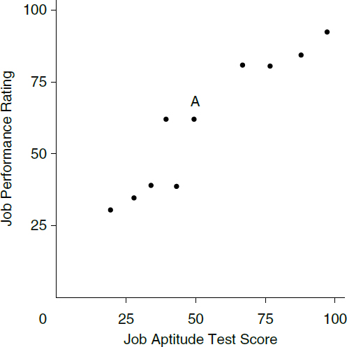
be relatively strong or relatively weak. If the relationship is sufficiently weak, there is effectively no correlation, as is illustrated in Figure 3(c).
Multiple regression analysis goes beyond simple correlation by deriving the “best fitting” linear function of all the covariates in predicting the dependent variable. For example, if average job performance ratings depend on aptitude test scores, age, and education, multiple regression analysis can use information about the joint behavior of job performance and the three explanatory variables in the observed sample to derive the best fitting linear function of aptitude test scores, age, and education in predicting job performance.
Many aspects of regression analysis can be illustrated in the case where there is only a single explanatory variable. A linear relationship between an explanatory variable X and a dependent variable Y is just the equation of a line:
| Y = a + bX | (1) |
In this equation, a is the intercept of the line (i.e., the height of the line when it intersects the y-axis with X = 0), and b is the slope (the change in the dependent variable associated with a 1-unit change in the explanatory variable). It is important to note the “1-unit change” interpretation, because sometimes the units of measurement change (e.g., from ounces to pounds), and in that case the
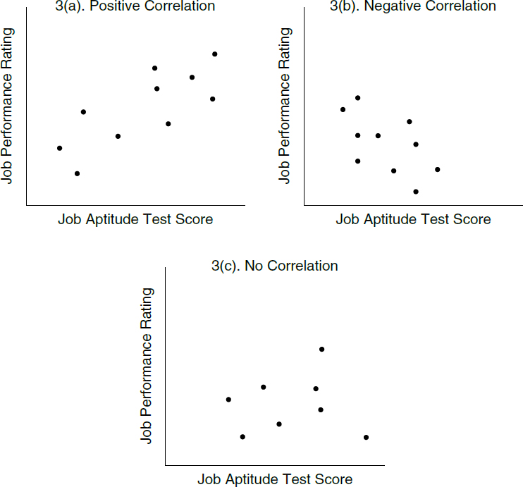
meaning of a “1-unit change” also changes. For example, if b is the slope when X is measured in pounds, then the slope when X is measured in ounces will be b/16, since each ounce is only 1/16 of a pound.
Unless Y is perfectly linearly related to X, equation (1) does not fully describe the determination of Y. Instead, there is a third term in the equation representing the part of Y that is not attributable to the linear effect of X:
| Y = a + bX + ε | (2) |
The term ε, usually called the residual term or the error term, incorporates all the determinants of Y apart from the intercept (also called a constant term) and
the linear effect of X. In many cases, an analyst will assume that the average value of the residual term is 0 for each value of X. In that case, the fact that there is a high or low value of X has no bearing on the likely sign (positive or negative) or magnitude of the other unobserved determinants of Y. As discussed above, however, in the interpretation of regression models, one of the critical issues is the plausibility of this assumption.
A linear regression model typically is estimated using the method of least squares (also known as ordinary least squares, or OLS), in which the values of the coefficients a and b are calculated so that the sum of the squared residual values (measured by the arrows shown in Figure 4) is made as small as possible. Note that by squaring the residuals, positive and negative deviations of the value of Y from its predicted value (a + bX) are given equal weight. Minimization of the squared residuals also means large deviations of Y from its predicted value receive substantially more weight in the determination of a and b than small deviations.
Figure 4, for example, shows the fitted regression line relating aptitude scores (the X variable) to job performance (the Y variable). When the aptitude test score is 0, the predicted (average) value of the job performance rating is the intercept, 18.4. Also, for each additional point on the test score, the job performance rating increases 0.73 units, which is given by the slope 0.73. Thus, the estimated regression line is139
139. In discussions of estimated regression models, it is standard to denote the predicted value with a carrot (or “hat”) symbol.

Multiple Regression Model
When there are an arbitrary number of explanatory variables, the linear regression model takes the following form:
| Y = β0 + β1X1 + β2X2 + ⋯ + βkXk + ε | (3) |
where Y represents the dependent variable, such as the salary of an employee, and X1 . . . Xk represent the explanatory variables (e.g., education, years of work experience, location in a major metropolitan area, etc.). As in equation (2) above, the error term ε represents the collective influence of all omitted factors influencing Y. Sometimes an analyst will assume that these factors are purely random and can be represented as independent observations drawn from a normal distribution with mean 0 and some standard deviation. Other times, an analyst will leave the precise distribution of ε unspecified.
In a multiple regression, each of the explanatory variables has its own coefficient (e.g., β1 for the first variable, β2 for the second).140 In addition, there is a constant or intercept term, β0, which has the interpretation of the expected value (or mean) of Y when all of the explanatory variables have a value of 0 (similar to the interpretation of the constant term a in equation (2) above). The full set of coefficients (also referred to as the parameters of the regression model) is usually estimated by ordinary least squares, which again selects the values to minimize the sum of the squared residuals.
Each coefficient βk measures how the dependent variable Y responds, on average, to a change in the corresponding covariate Xk, holding constant the effects of the other covariates. This can be seen mathematically from equation (3): When all other covariates are held constant, and the value of the residual term is also held constant, a 1-unit increase in the kth covariate will change the value of the dependent variable by an amount βk.
An important feature of the use of ordinary least squares to estimate the coefficients in equation (3) is that one can give a precise interpretation of how the estimated coefficients are obtained in such a way as to reflect the “holding constant” of the other covariates. Consider the following three-step procedure. First, calculate the residuals from a regression of Y on all covariates other than Xk. These residuals reflect the part of Y that cannot be explained by the other control variables. Second, calculate the residuals of a regression of Xk on all the other covariates. These residuals reflect the part of Xk that cannot be explained by the other control variables. Third and finally, regress the first residual variable on the second residual variable. The resulting coefficient will be identical to βk. Thus the coefficient in a multiple regression represents the slope of the line “Y, adjusted for all covariates other than Xk versus Xk adjusted for all the other covariates.”141
Most statisticians and applied economists use the least-squares regression technique because of its simplicity and its desirable statistical properties. As a result, it is also used frequently in legal proceedings.
140. The variables themselves can appear in many different forms. For example, Y might represent the logarithm of an employee’s salary, and X1 might represent the logarithm of the employee’s years of experience. The logarithmic representation is appropriate when Y increases exponentially as X increases—for each unit increase in X, the corresponding increase in Y becomes larger and larger. For example, if an expert were to graph the growth of the U.S. population (Y) over time (t), the following equation might be appropriate: log(Y) = β0 + β1log(t).
141. In econometrics, this is known as the Frisch-Waugh-Lovell theorem. Note that if Xk can be perfectly predicted by the other explanatory variables, then there will be no residuals to take to the third step—this is the extreme case of perfect multicollinearity.
Specifying the Regression Model
Suppose an expert wants to analyze the salaries of women and men at a large publishing house to discover whether a difference in salaries between employees with similar years of work experience provides evidence of discrimination.142 To begin with the simplest case, the salary in dollars per year, Y, represents the dependent variable to be explained, and X1 represents the number of years of experience of the employee explanatory variable. The regression model would be written
| Y = β0 + β1X1 + ε | (4) |
In equation (4), β0 and β1 are the parameters to be estimated from the data, and ε is the error term. The parameter β0 is the average salary of all employees with no experience. The parameter β1 measures the average effect of an additional year of experience on the average salary of employees.
Fitted Regression Line
Once the parameters in a regression equation have been estimated, the fitted values for the dependent variable can be calculated. If the estimated regression parameters, or regression coefficients, for the model in equation (3) are denoted as , ,…, , the fitted values for Y, denoted Ŷ, are
| (5) |
Figure 5 illustrates this for the example involving a single explanatory variable. The data are shown as a scatter of points; salary is on the vertical axis, and years of experience is on the horizontal axis. The estimated regression line is drawn through the data points. It is given by
| Ŷ = $15,000 + $2,000X1 | (6) |
Thus, the fitted value for the salary of individual i, who has X1i years of experience, will be given by
| (7) |
142. The regression results used in this example are based on data for 1,715 men and women; these results were used by the defense in a sex-discrimination case against the New York Times that was settled in 1978. Professor Orley Ashenfelter, Department of Economics, Princeton University, provided the data.
The intercept of the regression model represents the average value of the dependent variable when the explanatory variable or variables are equal to 0; the estimated intercept b0 is shown on the vertical axis in Figure 5. Similarly, the slope of the line measures the (average) change in the dependent variable associated with a unit increase in an explanatory variable; the estimated slope b1 also is shown. In equation (6), the intercept $15,000 indicates that employees with no experience earn $15,000 per year. The slope parameter implies that each year of experience adds $2,000 to an “average” employee’s salary.
Now, suppose that the salary variable is related simply to the sex of the employee. The relevant indicator variable, often called a dummy variable, is X2, which is equal to 1 if the employee is male, and 0 if the employee is female. Suppose the regression of salary Y on X2 yields the following result: Y= $30,449 + $10,979X2. The coefficient $10,979 measures the difference between the average salary of men and the average salary of women.143
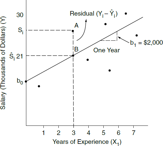
143. To understand why, note that when X2 = 0, the average salary for women is $30,449 + $10,979 × 0 = $30,449. Correspondingly, when X2 = 1, the average salary for men is $30,449 + $10,979 × 1 = $41,428. The difference—$41,428 − $30,449—is $10,979.
Regression residuals
Recall that for each data point, the regression residual is the difference between the actual value of the dependent variable and part of that value that is attributable to the explanatory variables. After a regression model has been estimated, the estimated regression residual () is the difference between the actual values and the fitted or predicted values from the estimated model. Suppose, for example, that we are studying an individual with three years of experience and a salary of $27,000. According to the estimated regression line in Figure 5, the predicted salary of an individual with three years of experience is $21,000. (This can also be interpreted as the expected salary that an individual with three years of experience would receive, since all the unexplained terms in the residual should on average take a value of 0.) Because the individual’s salary is $6,000 higher than the predicted salary from the model, the estimated residual (the individual’s salary minus the predicted salary, based on the estimated coefficients) is $6,000. In general, the estimated residual associated with a data point, such as Point A in Figure 5, is given by . Each data point in the figure has an estimated residual, which is the error made by the least-squares regression method for that individual.
Interaction terms
Models with interaction terms allow for the possibility that the effect of an explanatory variable on the dependent variable may vary in magnitude as the level of other explanatory variables changes. As a starting point, assume that the regression model takes the following form:
| Y = β0 + β1MALE + β2EXP + ε | (8) |
where Y is annual salary, MALE is equal to 1 for men and 0 for women, EXP represents years of job experience, and ε is the error term. The coefficient β1 measures the difference in average salary (across all experience levels) between men and women. In essence the inclusion of a dummy variable such as MALE allows for a parallel vertical shift in the regression line. The shift is parallel because the slope coefficient β2, which measures the effect of experience on salary, is the same for both males and females.
Now suppose that the regression model is expanded to take on the following form:
| Y = β0 + β1MALE + β2EXP + β3EXP × MALE + ε | (9) |
In this model, the coefficient β1 measures the difference in average salary (across all experience levels) between men and women for employees with no experience. The coefficient β2 measures the effect of experience on salary for women (when MALE = 0), and the interaction coefficient β3 measures the difference in the effect of experience on salary between men and women. It follows, for example, that the effect of one year of experience on salary for women is β2, whereas the comparable effect for men is β2 + β3.144
Interpreting regression results
To explain how regression results are interpreted, we can expand the earlier example associated with Figure 5 to consider the possibility of an additional explanatory variable—the square of the number of years of experience, X3. The X3 variable is designed to capture the fact that for most individuals, salaries increase with experience, but at a faster rate for people who first enter the labor market (with low levels of experience), and a lower rate for people with more experience. Thus, we might expect the estimated coefficient of X1 to be positive and the estimated coefficient of X3 to be negative.145
The estimated regression line using the third additional explanatory variable, as well as the first explanatory variable for years of experience (X1) and the dummy variable for male gender (X2), is
Ŷ= $14,085 + $2,323X1 + $1,675X2 − $36X3
The importance of including relevant explanatory variables in a regression model is illustrated by the change in the regression results after the X3 and X1 variables are added. The coefficient on the variable X2 measures the difference in the salaries of men and women while controlling for the linear and quadratic effects of experience. The differential of $1,675 is substantially lower than the previously measured differential of $10,979. Clearly, failure to control for job experience in this example leads to an overstatement of the difference in salaries between men and women.
Now consider the interpretation of the explanatory variables for experience, X1 and X3. The positive sign on the X1 coefficient shows that salary increases with experience. The negative sign on the X3 coefficient indicates that the rate of
144. Estimating a regression in which there are interaction terms for all explanatory variables, as in equation (9), is essentially the same as estimating two separate regressions, one for men and one for women.
145. A model that includes a variable and its square is often referred to as a quadratic specification. Thus, the equation on this page would be referred to as a model that includes controls for “a quadratic in experience.”
salary increase diminishes with experience (as expected). To determine the combined effect of the variables X1 and X3, some simple calculations can be made.146 For example, consider how the average salary of women (X2 = 0) changes with the level of experience. As experience increases from zero to one year, the average salary increases by $2,287 ($2,323 − $36), from $14,085 to $16,372. However, women with two years of experience earn only $2,215 more than women with one year of experience, and women with three years of experience earn only $2,143 more than women with two years.147 Figure 6 illustrates the results: The regression line shown is for women’s salaries; the corresponding line for men’s salaries would be parallel and $1,675 higher.
The problem of omitted variables
A major problem confronting the interpretation of regression models is the possibility that some of the unobserved or omitted factors included in the error term are in fact correlated with the included variables. For example, consider an analysis of the effect of having attended a prestigious law school on the earnings of attorneys 10 years after completion of their law degrees. The available dataset
146. More formally, consider a model that relates a dependent variable to some variable Z with a coefficient of β1 and to its square (Z2) with a coefficient of β2 (i.e., Y = β1Z + β2Z2 + . . .). The marginal effect of a small increase in Z on the predicted value of the dependent variable is β1 + 2β2Z, which is the derivative of the quadratic expression.
147. These numbers can be calculated by substituting different values of X1 and X3 in the previous equation.
includes a sample of students who attended different law schools, a measure (Y) of their annual salary in the tenth year post-graduation, an indicator (X1) for having attended a “top 20” law school; an indicator for female gender (X2), and an indicator (X3) for whether their undergraduate degree was in a STEM (Science, Technology, Engineering, and Mathematics) field or not. The expert intends to interpret the coefficient on attending a top 20 school as the causal effect of the superior training and network opportunities afforded by such a school, as part of litigation over the admission rules used by certain schools.
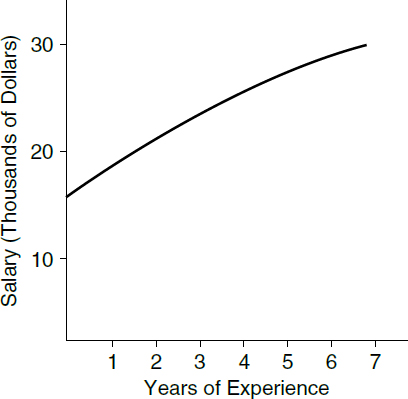
The proposed regression model takes the following form:
| Y = β0 + β1X1 + β2X2 + β3X3 + ε | (10) |
Included in the error term ε are all the other unmeasured factors affecting salary, apart from the three covariates. Some of these factors, such as interest in pursuing a public interest law career, may negatively affect salary, while others, like ambition or ability, may positively affect salary. Moreover, it is likely that the average value of ε is different for students who attended a top 20 program versus those who did not. How does this affect the estimates of the coefficient β1?
It turns out there is a very simple answer, at least conceptually. Consider the hypothetical regression model relating ε to the three covariates:
| ε = λ0 + λ1X1 + λ2X2 + λ3X3 + ξ | (11) |
Here, the coefficients λ1, λ2, and λ3 represent the effects of attending an elite school, being female, or having a STEM undergraduate degree on the combination of omitted factors that are included in ε. For example, if λ1 > 0, then attending an elite school is associated, on average, with a more positive combination of omitted factors. Note that if the error term in equation (10) is truly random, and independent of the included covariates, then all the λ coefficients in (11) will be zero. Alternatively, if X1 were randomly determined by an admissions lottery, then λ1 would be zero, since there is no information in a randomized variable that can be used to predict other variables.
When the regression model (10) is estimated by OLS, the coefficients of the included covariates will incorporate both the true causal effects of the covariates (i.e., the β’s), and the effect of the covariates in predicting ε (i.e., the λ’s):
| Y = (β0 + λ0) + (β1 + λ1)X1 + (β2 + λ2)X2 + (β3 + λ3)X3 + ξ | (12) |
Notice that the error in this model is the error from the hypothetical regression model (11): this is the part of ε that cannot be predicted by the included covariates. Equation (12) says that in estimating a multiple regression of salaries on elite school status, gender, and STEM major, the coefficient associated with attending an elite school is actually β1 + λ1, reflecting the fact that attending an
elite law school has a direct effect on salary, β1, holding constant the other controls and all the unobservable factors in ε, plus an indirect effect arising because on average people who attend an elite law school have different values of ε. This second term, λ1, is known as omitted-variables bias.
To summarize, if one estimates a multiple regression model relating an outcome to a set of observed covariates, the estimated coefficients will be estimates of the combined effect of the causal coefficients in the intended model and the coefficients that arise in trying to predict whatever is left in the error term in this model. This happens because the actual regression coefficients are algorithmically selected to form the best possible estimate of Y, given the observed covariates. In choosing the coefficients, the OLS algorithm does not distinguish between the intended causal effects in the model and the potential role of the covariates in predicting the residual component in the model.
Although equations (10)–(12) provide a useful framework for thinking about omitted-variables biases, it is important to keep in mind that the hypothetical regression (11) cannot be estimated, because we cannot actually see the value of ε. Nevertheless, analysts often present detailed discussions of the likely sign (and less commonly, the magnitude) of the coefficients in the hypothetical regression. If it can be argued, for example, that λ1 is almost surely positive, then one can infer that the estimated effect of attending an elite law school from a model based on (10) is almost surely upward biased as an estimate of β1. In addition, sometimes information from another sample can be used to help assess the signs and magnitudes of omitted-variables biases. For example, suppose information from a previous study shows that higher LSAT scores are associated with higher salaries and that information is available on the average LSAT scores of students attending different law schools. From these sources it might be possible to make an educated guess about a plausible magnitude for λ1.
Causal Modeling
Pre/Post Comparisons
Concerns over omitted-variables bias in regression models have led to the development of alternative regression-based approaches for estimating the causal effect of a variable of interest. These approaches typically focus on situations where the value of the explanatory variable of interest changes discretely for a known reason (e.g., a political decision).148 For example, suppose one is interested in understanding the effect of more intensive policing on crime. One might then focus on cases where a new policing program (e.g., New York City’s “stop and frisk” program) is introduced. If data on crime rates are available from both before and after
148. Sometimes these changes are referred to as quasi-experiments or natural experiments.
the introduction, a pre/post estimate of the effect of the policy can be constructed from the change in the average number of crimes per day following the implementation of the new policy.
In a pre/post research design (and in related difference-in-differences designs), it is necessary to distinguish between the two separate dimensions over which the data are observed. One dimension is across different units, indexed by the subscript i (e.g., in a study of policing and crime, the units of observation may be police precincts); the other is over time (e.g., different months or years), indexed by the subscript t. Using this notation, let Yit represent the outcome of interest observed for unit i in period t. Assume that a new program or intervention is initiated at time t = 1. In earlier periods (t = 0, t = −1, t = −2, . . .), the program was absent; in all periods on or after t = 1, the program is in place. A very simple model for Yit is one that includes a constant and an indicator for post-intervention periods, Postt = 0 if t ≤ 0, and Postt = 1 if t ≥ 1:
| Yit = β0 + β1Postt + εit. | (13) |
This simple model implies that in all periods up to period 0,
| Yit = β0 + εit | (14) |
whereas in all later periods t = 1, 2, . . . ,
| Yit = β0 + β1 + εit. | (15) |
Setting t = 1 in equation (15) and setting t = 0 in equation (14) and subtracting, the change in the outcome for unit i from period 0 to period 1 is
| ΔYi = Yi1 − Yi0 = β1 + εi1 − εi0. | (16) |
Treating εi1 − εi0 as a residual, equation (16) is the simplest possible regression model, with a constant term and no other covariates. The OLS estimate of β1 in such a model is exactly the mean change in the outcome across all the units in the sample, that is,
| (17) |
where Mean(Y) denotes the mean value of the variable Y in the sample.
To interpret equation (17), note that Mean(ΔYi) = Mean(Yi1) − Mean(Yi0). In a pre/post design, the mean outcome in the post period is compared to the mean outcome in the pre period. If the mean value of the outcome does not change after the intervention, the estimated effect of the intervention is 0. If the mean outcome rises (falls), then will be positive (negative). Conceptually, a pre/post
design is using the mean of the outcome in the pre-intervention period as an estimate of what the mean would have been in the absence of the intervention. This is known as the counterfactual mean in applied economics, or the but-for mean in legal discussions. The difference between the actual mean in the post-intervention period and the counterfactual mean is the estimated effect of the intervention.
If data were only available from the period after the start of the intervention, an alternative approach would be to try to find another set of units that have not adopted the intervention and use the mean of the outcomes for this “comparison group” as a counterfactual. In the policing example, suppose that some precincts adopt the new program, and some do not. Then one might consider using the average crime rates for precincts that did not adopt the policy as the counterfactual for those that did.149 A concern with this alternative approach is that there may be differences between units that adopted the new program and units that did not, raising the possibility of omitted-variables bias. In a pre/post design, the counterfactual is based on the average outcomes of the same units before they implemented the intervention. In some cases, this counterfactual will be more compelling.
The potential advantages of a pre/post design are illustrated by decomposing εit, the error term in equation (13), into two parts: a part αi that is constant over time, representing the mean value of all the εit’s for unit i, and the deviation of εit from its mean value in period t,
| εit = αi + vit | (18) |
For example, in a study of crime and policing where i indexes different precincts and t has two values, t = 0 and t = 1, the error εit from the model in equation (11) has the interpretation of the deviation in the crime rate in a precinct i in period t from the average crime rate in the city in the same period. One might expect certain precincts to have higher average crime rates in both periods, and others to have lower crime rates. Such differences in average rates would be reflected in the αi component of equation (18), whereas unexplained fluctuations in crime from period to period in the same precinct would be reflected in the vit component. From equation (18) it follows that the difference in εit between period 0 and period 1, which is the error term in equation (16), is
| εi1 − εi0 = vi1 − vi0 | (19) |
Differencing eliminates the time-invariant component of εit, leaving a new error term that is less likely to be affected by omitted-variable biases, since all the
149. This would replace equation (13) with an alternative model: Yi = β0 + β1Adopti + εi, where Adopti is an indicator variable equal to 1 for precincts that adopted the policy and 0 for those that did not. In such a model, the OLS estimate of the coefficient β1 is = Mean(Y | Adopti = 1) − Mean(Y | Adopti = 0), where Mean(Y | C) denotes the mean in the sample among units for which condition C is true.
permanent factors that differ across units are removed through the differencing process.
Nevertheless, a simple pre/post design has an important limitation: any change that affects the average value of the outcome between period 0 and period 1 is attributed to the intervention. In many situations, the mean value of an outcome changes over time for reasons that have nothing to do with the intervention or change in policy under study. One way to check whether such factors are present is to construct average differences in the outcome for earlier periods and verify that these are all very close to zero. For example, equation (13) implies that the lagged difference in outcomes ΔYi(−1) is determined by
| ΔYi(−1) = Yi0 − Yi(−1) = εi0 − εi(−1). | (20) |
The same arguments that support the contention that the error term εi1 − εi0 in equation (16) has a mean value of 0, so that Mean(ΔYi) provides a good estimate of β1, imply that the error term in equation (20) also has a mean value of 0. Thus, Mean(ΔYi(−1)) should be very close to 0. Indeed, the mean values of the changes in the outcome for all periods where there was no change in policy should be close to 0. In the absence of evidence that this is true, a simple pre/post design is not very credible.
Difference in Differences
A natural way to address the presence of unmeasured factors that are changing over time and confounding the interpretation of a simple pre/post design is to compare the change in the outcome for units where the new program was adopted to the change in the outcome over the same period for units that did not adopt the program. This is the difference-in-differences approach.
To spell this out, call the treatment group the set of units where the program is adopted between period 0 and period 1; call the other set of units the comparison group, and let Ti be an indicator variable that is equal to 1 for units in the treatment group. Suppose that data are only observed in periods 0 and 1. Then, the difference-in-differences model can be written as a multiple linear regression model of the form
| Yit = β0 + β1Ti × Postt + β2Ti + β3Postt + εit | (21) |
The key coefficient in this model is β1, the coefficient on the interaction between the indicator for the treatment group and the indicator for period 1 (the post period).
To understand this equation, notice that for units with Ti = 0, it implies
| Yit = β0 + β3Postt + εit | (22) |
Thus, the change in outcomes for units in the comparison group is
| ΔYi = Yi1 − Yi0 = β3 + εi1 − εi0 | (23) |
The inclusion of the term β3Postt in equation (22) captures the possibility that even in the comparison group, unobserved factors can change between period 0 and period 1. Assuming the mean value of εi1 − εi0 is 0 for comparison units, the expected average change in the outcome in the comparison group will be β3.150 For units in the treatment group, equation (21) implies
| Yit = (β0 + β2) + (β1 + β3)Postt + εit | (24) |
Thus, the change in outcomes for units in the treatment group is
| ΔYi = (β1 + β3) + εi1 − εi0 | (25) |
Assuming that the mean value of εi1 − εi0 is 0 for units in the treatment group, the expected average change in the outcome in the treatment group will be β1 + β3, which is a combination of the change experienced by the comparison group, β3, and the effect of the program, β1. In fact, the OLS estimate of β1 in the difference-in-differences model (21) is exactly
| (26) |
where Mean(ΔYi |Ti = 1) denotes the mean in the subsample with Ti = 1 (i.e., among the treatment group), and Mean(ΔYi |Ti = 0) denotes the mean in the subsample with Ti = 0 (i.e., among the comparison group).
The critical assumption in a difference-in-differences design is that in the absence of the program, the mean change in outcomes for the treatment group and comparison groups would have been the same. Under that assumption, the mean change for the comparison group forms a counterfactual for the change that would have occurred in the treatment group in the absence of the program. As noted previously, this assumption is sometimes referred to as a parallel trends assumption. With only two periods of data, it cannot be directly evaluated. If there are additional periods of data, however, parallel trends can be assessed by forming differences in differences for other periods that do not overlap with the start of the program. These should all be close to zero. Visually, a graph of the mean outcomes for the treatment group over a sequence of periods (for example, t = −2, −1, 0, 1, 2) should show that the the gap between the treatment means and
150. To be precise, the “expected average change” means the mathematical expectation of the sample average change in the outcome.
comparison means is stable prior to the program date, then shifts discretely between period 0 and 1, reflecting the treatment effect, then stabilizes again.
Another way of thinking about the validity of a difference-in-differences specification is to ask whether the choice of the pre-treatment period matters. For example, consider an evaluation of a state law that liberalizes state divorce law. A difference-in-differences approach to measuring the effect of the law would be to compare the change in divorce rates from some year prior to the law to the year after the law changed in the “treatment” state (the state that passed the new law) relative to the change in divorce rates in a “comparison” state. If the assumptions of a difference-in-differences specification are correct, then the relative change in divorce rates in the treated state relative to the comparison state should not depend on the particular year that is selected as the benchmark prior to the law change. Under those assumptions, the difference in divorce rates in the treated and comparison states can be expected to be similar in all the years prior to the new law. As a result, choosing one particular year as a benchmark versus another will not matter. Graphically, this requires that the year-to-year changes in divorce rates in the treated state and the comparison state are the same, and a plot of the divorce rates prior to the law change would appear as two parallel lines. This is the origin of the term parallel trends.
A common scenario where the parallel trends assumption may fail is one in which the timing of the program is correlated with the trend in recent outcomes for the treatment group. For example, Ashenfelter (1978) noted that people who entered government retraining programs had temporarily depressed earnings in the period before entry, driven by recent job losses or other problems—the Ashenfelter dip.151 Building on equation (18), this suggests that program participants may be particularly likely to have large negative values of vi0 (the period-specific part of their earnings residual in the period just prior to the program). In that case, the mean value of the error term εi1 − εi0 = vi1 − vi0 in equation (25) will be positive, implying that
| Mean(ΔYi|Ti = 1) = β1 + β3 + Mean(εi1 − εi0|Ti = 1) > β1 + β3 | (27) |
causing a difference-in-differences estimator to overstate the effect of the program. The possibility of such pre-trends can be evaluated empirically by examining the mean outcomes of the treatment and comparison groups in the periods before the start of the program and making sure that the parallel trends assumption is valid.
151. Ashenfelter, supra note 94.
Instrumental Variables
An alternative method that is widely used to address omitted variables problems in regression models is instrumental variables (IV). Consider the case where an expert has posited a model relating an outcome Y to an observed explanatory variable:
| Yi = β0 + β1Xi + εi | (28) |
For clarity, subscripts indicate the different units (indexed by i) in the sample. The expert wants to give a causal interpretation of the coefficient β1. Specifically, in the expert’s model, β1 represents the effect of a unit change in X on the average or expected value of the outcome, holding constant all other unmeasured/unobserved determinants of Y. Such an equation is known as the structural model in IV and related settings. The problem is that, if this structural equation is estimated by OLS, the estimate will incorporate both the desired causal effect and any potential omitted variable bias that arises because Xi is potentially correlated with some of the factors included in the error εi. This omitted-variable bias is sometimes called a simultaneity bias or endogeneity bias—particularly in cases where there is feedback from Yi to Xi, as discussed in the section titled “Instrumental Variables Design” above. Whatever the source of the potential correlation between Xi and εi, however, it can be analyzed in the omitted variables framework of equations (10)–(12).
The objective of IV estimation is to isolate the part of the variation in Xi attributable to variation in some other variable, Zi (the instrumental variable or the instrument), and use only that variation in estimating the effect of Xi on Yi. An appropriate instrumental variable has to satisfy three assumptions: (1) it has an effect on Xi, so there is a component of Xi that can be attributed to Zi; (2) it is uncorrelated with εi, the unobserved determinants of Yi; and (3) it has no direct effect on the outcome Yi. An example of an instrumental variable that satisfies these requirements is a randomly assigned lottery outcome. For example, in a study of the effect of attending a charter school on test scores, the analysis showed that if access to over subscribed charter schools is determined by lottery, then an appropriate instrumental variable is an indicator for whether a student was assigned to the charter school by the admission lottery.152
The IV method involves estimating two regression models. The first-stage model is a linear regression relating the variable of interest (Xi) to the instrumental variable:
| Xi = π0 + π1Zi + ui | (29) |
152. See generally Chabrier et al., supra note 104.
From this model it is possible to form the predicted values of Xi based only on Zi:
| (30) |
The second-stage model is a linear regression of the outcome on the predicted values of Xi:
| (31) |
The OLS estimate of the coefficient of in the second-stage model, , is the IV estimate of β in the structural model (28). Note that since only depends on Zi, the second-stage equation measures the effect of the part of that is determined by Zi on the outcome variable.
The IV estimate can be derived in another way. Substituting the first-stage equation (29) into the structural equation (28) yields an equation relating Y to Z:
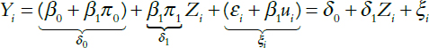 | (32) |
This equation, known as the reduced-form model, can be estimated by OLS without concern about omitted variables bias because, under the assumption that Zi is a valid instrumental variable, it is uncorrelated with ξi.153 But equation (32) shows that the coefficient of the instrumental variable in the reduced-form model is δ1 = β1π1. This occurs because under assumption #3 for a valid instrumental variable, the only way that Zi affects Yi is indirectly, through its effect on Xi. Since Zi affects Xi with a coefficient of π1 in the first-stage model, and Xi affects Yi with a coefficient of β1 in the structural model, the reduced-form effect of Zi on Yi is the product of these two coefficients. This reasoning suggests that one could obtain an estimate of β1 by dividing the estimated reduced-form coefficient, , by the estimated first-stage coefficient . And in fact this ratio is exactly the IV estimate:
| (33) |
The expression for the IV estimate in equation (33) is particularly insightful in the case where Xi is a dummy variable indicating participation in a program or
153. Under assumption #2 for a valid instrumental variable, Zi is uncorrelated with εi. Moreover, the error in the first-stage equation ui, is necessarily uncorrelated with the explanatory variable in that model, by a fundamental property of least squares. Thus Zi is uncorrelated with the composite error in the reduced-form model, ξi = εi + β1ui.
intervention (for example, enrollment in a charter school), and Zi is also a dummy variable, indicating a condition that partly determines program participation (for example, whether student i was assigned to the charter school by lottery). In this case, the first-stage coefficient is the difference in program participation rates between units with Zi equal to 0 or 1:
| (34) |
and the reduced-form coefficient is the difference in the mean of the outcome variable (e.g., an end-of-year test score) for the same two groups:
| (35) |
Thus, equation (33) implies that the IV estimator for the effect of program participation on the outcome is
| (36) |
The IV estimator takes the difference in mean outcomes between the group with Zi = 1 and the group with Zi = 0, and divides this by the difference in the fraction who participated in the program when Zi was 1 or 0. Intuitively, the IV estimator is simply creating a per unit estimate of the treatment effect of the intervention, based on the differences between groups with different values of Zi.
Determining the Precision of the Regression Results
Least squares regression algorithms provide not only parameter estimates that indicate the direction and magnitude of the effect of a change in the explanatory variable on the dependent variable, but also an estimate of the reliability of the parameter estimates and a measure of the overall goodness of fit of the regression model. Each of these factors is considered in turn.
Standard Errors of the Coefficients and t-Statistics
Estimates of the true but unknown parameters of a regression model are numbers that depend on the sample of observations under study. If a different sample
were used, a different estimate would be calculated.154 If the expert continued to collect more and more samples and generated additional estimates, as might happen when new data became available over time, the estimates of each parameter would follow a probability distribution. This probability distribution can be summarized by a mean and a measure of dispersion around the mean, a standard deviation, which usually is referred to as the standard error of the coefficient, or the standard error (SE).155
Suppose, for example, that an expert is interested in estimating the average price paid for a gallon of unleaded gasoline by consumers in a particular geographic area of the United States at a particular point in time. The mean price for a sample of 10 gas stations might be $1.25, while the mean for another sample might be $1.29, and the mean for a third, $1.21. On this basis, the expert also could calculate the overall mean price of gasoline to be $1.25 and an estimate of the standard deviation to be $0.04.
Least-squares regression generalizes this result, by calculating means whose values depend on one or more explanatory variables. The standard error of a regression coefficient tells the expert how much parameter estimates are likely to vary from sample to sample. The greater the variation in parameter estimates from sample to sample, the larger the standard error and consequently the less reliable the regression results. Small standard errors imply results that are likely to be similar from sample to sample, whereas results with large standard errors show more variability.
Under appropriate assumptions, the ordinary least-squares estimators provide “best” determinations of the true underlying parameters.156 In fact, OLS has several desirable properties. First, assuming that the error term in the regression model is uncorrelated with the covariates, least squares estimators are unbiased. Intuitively, this means that if the regression were calculated repeatedly with different samples, the average of the many estimates obtained for each coefficient would be the true parameter. Second, under the same assumption, least-squares estimators are consistent; if the sample were very large, the estimates obtained would come close to the true parameters. Third, least squares is efficient, in that its estimators have the smallest variance among all (linear) unbiased estimators.
If the further assumption is made that the probability distribution of each of the error terms is known, statistical statements can be made about the precision
154. The least squares formula that generates the estimates is called the least squares estimator, and its values vary from sample to sample.
155. See David H. Kaye & Hal S. Stern, Reference Guide on Statistics and Research Methods, “Randomized Controlled Experiments” section, in this manual.
156. The necessary assumptions of the regression model include (a) the model is specified correctly, (b) errors associated with each observation are drawn randomly from the same probability distribution and are independent of each other, (c) errors associated with each observation are independent of the corresponding observations for each of the explanatory variables in the model, and (d) no explanatory variable is correlated perfectly with a combination of other variables.
of the coefficient estimates. For relatively large samples (often, thirty or more data points will be sufficient for regressions with a small number of explanatory variables), the probability that the estimate of a parameter lies within an interval of 1.96 standard errors around the true parameter is approximately .95, or 95%. A frequent, although not always appropriate, assumption in statistical work is that the error term follows a normal distribution, from which it follows that the estimated parameters are normally distributed. The normal distribution has the property that the area within 1.96 standard errors of the mean is equal to 95% of the total area. Note that the normality assumption is not necessary for least squares to be used, because most of the properties of least squares apply regardless of normality.
In general, for any parameter estimate , the expert can construct an interval around such that if the sampling procedure were conducted 100 times, approximately 95 of the resulting intervals would be expected to contain the true population mean. The 95% confidence interval157 is given by158
| (37) |
The expert can test the hypothesis that a parameter is equal to 0 (often stated as testing the null hypothesis) by looking at its t-statistic, which is defined as
| (38) |
If the t-statistic is less than 1.96 in magnitude, the 95% confidence interval around must include 0.159 Because this means that the expert cannot reject the hypothesis that β equals 0, the estimate, whatever it may be, is said to be not statistically significant. Conversely, if the t-statistic is greater than 1.96 in absolute value, the expert concludes that the true value of β is unlikely to be 0 (intuitively, is “too far” from 0 to be consistent with the true value of β being 0). In this case, the expert rejects the hypothesis that β equals 0 and calls the estimate statistically significant. If the null hypothesis β equals 0 is true, using a 95% confidence level will cause the expert to falsely reject the null hypothesis 5% of the time. Consequently, results often are said to be significant at the 5% level.160
157. Confidence intervals are used commonly in statistical analyses because the expert can never be certain that a parameter estimate is equal to the true population parameter.
158. If the number of data points in the sample is small (perhaps less than 30), the 1.96 number must be adjusted upward.
159. The t-statistic applies to any sample size. As the sample size increases, the underlying distribution, which is the source of the t-statistic (Student’s t-distribution), approximates the normal distribution.
160. A t-statistic of 2.57 in magnitude or greater is associated with a 99% confidence level, or a 1% level of significance, that includes a band of 2.57 standard deviations on either side of the estimated coefficient.
As an example, consider a more complete set of regression results associated with the salary regression described earlier:
| (39) |
The standard error of each estimated parameter is given in parentheses directly below the estimated coeffcient, and the corresponding t-statistics appear below the standard error values.
Consider the coefficient on the dummy variable X2, representing the sex of a worker. It indicates that $1,675 is the best estimate of the mean salary difference between men and women. However, the standard error of $1,435 is large in relation to its coefficient $1,675. Because the standard error is relatively large, the range of possible values for measuring the true salary difference, the true parameter, is great. In fact, a 95% confidence interval is given by the range negative $1,138 to positive $4,488. In other words, the expert can have 95% confidence that the true value of the coefficient lies between –$1,138 and $4,488. Because this range includes 0, the effect of sex on salary is said to be insignificantly different from 0 at the 5% level. The t value of 1.2 is equal to $1,675 divided by $1,435. Because this t-statistic is less than 1.96 in magnitude (a condition equivalent to the inclusion of a 0 in the above confidence interval), the sex variable again is said to be an insignificant determinant of salary at the 5% level of significance.
Note also that experience is a highly significant determinant of salary, because both the X1 and the X3 variables have t-statistics substantially greater than 1.96 in magnitude. More experience has a significant positive effect on salary, but the size of this effect diminishes significantly with experience.
Goodness of Fit
Reported regression results usually contain not only the point estimates of the parameters and their standard errors or t-statistics, but also other information that tells how closely the regression line fits the data. One statistic, the standard error of the regression (SER), is an estimate of the overall size of the regression residuals.161 An SER of 0 would occur only when all data points lie exactly on the regression line—an extremely unlikely possibility. Other things being equal, the larger the SER, the poorer the fit of the data to the model.
161. More specifically, it is a measure of the standard deviation of the regression error ε. It sometimes is called the root mean square error of the regression line.
For a normally distributed error term, the expert would expect approximately 95% of the data points to lie within two SERs of the estimated regression line, as shown in Figure 7.

R-squared (R2) is a statistic that measures the percentage of variation in the dependent variable that is accounted for by all the explanatory variables.162 Thus, R2 provides a measure of the overall goodness of fit of the multiple regression equation. Its value ranges from 0 to 1. An R2 of 0 means that the explanatory variables explain none of the variation of the dependent variable; an R2 of 1 means that the explanatory variables explain all the variation. The R2 is .56. This implies that the three explanatory variables explain 56% of the variation in salaries.
What level of R2, if any, should lead to a conclusion that the model is satisfactory? Unfortunately, there is no clear-cut answer to this question because the magnitude of R2 depends on the characteristics of the data being studied and whether the data vary over time or over individuals. Typically, an R2 is low in cross-sectional studies in which differences in individual behavior are explained. It is likely that these individual differences are caused by many factors that cannot be measured. As a result, the expert cannot hope to explain most of the variation. In time-series studies, in contrast, the expert is explaining the movement of aggregates over time. Because most aggregate time series have substantial
162. The variation is the square of the difference between each Y value and the average Y value, summed over all the Y values.
growth, or trend, in common, it will not be difficult to “explain” one time series using another time series, simply because both are moving together. It follows as a corollary that a high R2 does not by itself mean that the variables included in the model are the appropriate ones.
Courts should be reluctant to rely solely on a statistic such as R2 to choose one model over another. Alternative procedures and tests are available.163 When utilizing probit or logit models, the R2 is especially problematic, since (with the dependent variable taking on only two values) predictions will be spread across the 0–1 interval with relatively few values typically being close to either 0 or 1. As a result, R2 values will be relatively low whether the estimated model coefficients are informative or not. One more instructive measure is the percentage of correct classifications with the prediction being 1 if the predicted value is greater than .5 and 0 otherwise. An alternative measure is a quasi-R-squared measure based on the log likelihood of the estimated model, relative to that of a model with no covariates.
Sensitivity of Least-Squares Regression Results
The least-squares regression line can be sensitive to extreme data points. This sensitivity can be seen most easily in Figure 8. Assume initially that there are only three data points, A, B, and C, relating information about X1 to the variable Y. The least-squares line describing the best-fitting relationship between Points A, B, and C is represented by Line 1. Point D is called an outlier because it lies far from the regression line that fits the remaining points. When a new, best-fitting least-squares line is re estimated to include Point D, Line 2 is obtained. Figure 8 shows that the outlier, Point D, is an influential data point, because it has a dominant effect on the slope and intercept of the least-squares line. Because least squares minimizes the sum of squared deviations, the sensitivity of the line to individual points sometimes can be substantial.164
163. These include F-tests and specification error tests. See Pindyck & Rubinfeld, supra note 23, at 88–95, 128–36, 194–98.
164. This sensitivity is not always undesirable. In some instances, it may be much more important to predict Point D when a big change occurs than to measure the effects of small changes accurately.

What makes the influential data problem even more difficult is that the effect of an outlier may not be seen readily if deviations are measured from the final regression line. The reason is that the influence of Point D on Line 2 is so substantial that its deviation from the regression line is not necessarily larger than the deviation of any of the remaining points from the regression line.165 Although they are not as popular as least squares, alternative estimation techniques that are less sensitive to outliers, such as robust estimation, are available. Alternatively, if the sample is relatively large, an expert may choose to remove the outliers before estimating the model.
165. The importance of an outlier also depends on its location in the dataset. Outliers associated with relatively extreme values of explanatory variables are likely to be especially influential. See, e.g., Fisher v. Vassar College, 70 F.3d 1420, 1436 (2d Cir. 1995) (court required to include assessment of “service in academic community,” because concept was too amorphous and not a significant factor in tenure review), rev’d on other grounds, 114 F.3d 1332 (2d Cir. 1997) (en banc). Conclusory statements of an outlier’s impact are insufficient. See In re Nektar Therapeutics Sec. Litig., 34 F.4th 828, 836 (9th Cir. 2022) (“[t]he complaint does not allege with specificity what the Phase 1 EXCEL results would have been without outlier data”).
A Hypothetical Example
Jane Thompson filed suit in federal court alleging that officials in the police department discriminated against her and a class of other female police officers in violation of Title VII of the Civil Rights Act of 1964, as amended. On behalf of the class, Officer Thompson alleged that she was paid less than male police officers with equivalent skills and experience. Both the plaintiff and the defendant used expert economists with econometric expertise to present statistical evidence to the court in support of their positions.
The plaintiff’s expert pointed out that the mean salary of the 40 female officers was $30,604, whereas the mean salary of the 60 male officers was $43,077. To show that this difference was statistically significant, the expert put forward a regression of salary (SALARY) on a constant term and a dummy indicator variable (FEM) equal to one for each female and zero for each male. The results were as follows:
SALARY = $43,077 − $12,373 × FEM
St. Error ($1,528) ($2,416)
p-value <.01 <.01
R2 = .22
The −$12,373 coefficient on the FEM variable measures the mean difference between male and female salaries. Because the standard error is approximately one-fifth of the value of the coefficient, this difference is statistically significant at the 5% (and indeed at the 1%) level. If this is an appropriate regression model (in terms of its implicit characterization of salary determination), one can conclude that it is highly unlikely that the difference in salaries between men and women is due to chance.
The defendant’s expert testified that the regression model put forward was the wrong model because it failed to account for the fact that males (on average) had substantially more experience than females. The relatively low R2 was an indication that there was substantial unexplained variation in the salaries of male and female officers. An examination of data relating to years spent on the job showed that the average male experience was 8.2 years, whereas the average for females was only 3.5 years. The defense expert then presented a regression analysis that added an additional explanatory variable (i.e., a covariate), the years of experience of each police officer (EXP).
The new regression results were as follows:
SALARY = $28,049 − $3,860 × FEM + $1,833 × EXP
St. Error ($2,513) ($2,347) ($265)
p-value <.01 <.11 <.01
R2 = .47
Experience is itself a statistically significant explanatory variable, with a p-value of less than .01. Moreover, the difference between male and female salaries, holding experience constant, is only $3,860, and this difference is not statistically significant at the 5% level. The defense expert was able to testify on this basis that the court could not rule out alternative explanations for the difference in salaries other than the plaintiff’s claim of discrimination.
The debate did not end here. On rebuttal, the plaintiff’s expert made three distinct points. First, whether $3,860 was statistically significant or not, it was practically significant, representing a salary difference of more than 10% of the mean female officers’ salaries. Second, although the result was not statistically significant at the 5% level, it was significant at the 11% level.
Third, and most importantly, the expert testified that the regression model was not correctly specified. Further analysis by the expert showed that the value of an additional year of experience was $2,333 for males on average, but only $1,521 for females. Based on supporting testimonial experience, the expert testified that one could not rule out the possibility that the mechanism by which the police department discriminated against females was by rewarding males more for their experience than females. The expert made this point clear by running an additional regression in which a further covariate was added to the model. The new variable was an interaction variable, measured as the product of the FEM and EXP variables. The regression results were as follows:
SALARY = $35,122 − $5,250 × FEM + $2,333 × EXP − $812 × FEM × EXP
St. Error ($2,825) ($3,347) ($265) ($185)
p-value <.01 <.11 <.01 <.01
R2 = .65
The plaintiff’s expert noted that for all males in the sample, FEM = 0, in which case the regression results are given by the equation
SALARY = $35,122 + $2,333 × EXP
However, for females, FEM = 1, in which the corresponding equation is
SALARY = $29,872 + $1,521 × EXP
It appears, therefore, that females are discriminated against not only when hired (i.e., when EXP = 0), but also in the reward they get as they accumulate more experience.
The debate between the experts continued, focusing less on the statistical interpretation of any one regression model, but more on the model choice itself, and not simply on statistical significance, but also to practical significance.
Glossary of Terms
alternative hypothesis. See hypothesis test.
association. The degree of statistical dependence between two or more events or variables. Events are said to be associated when they occur more frequently together than one would expect by chance.
bias. Any effect at any stage of investigation or inference tending to produce results that depart systematically from the true values (i.e., the results are either too high or too low). A biased estimator of a parameter differs on average from the true parameter.
coefficient. An estimated regression parameter.
consistent estimator. An estimator that tends to become more and more accurate as the sample size grows.
correlation. A statistical means of measuring the linear association between variables. Two variables are correlated positively if, on average, they move in the same direction; two variables are correlated negatively if, on average, they move in opposite directions.
covariate. A variable that is possibly predictive of an outcome under study; an explanatory variable.
cross-sectional analysis. A type of analysis in which each data point is associated with a different unit of observation (e.g., an individual or a firm) measured at a particular point in time.
degrees of freedom (DF). The number of observations in a sample minus the number of estimated parameters in a regression model. A useful statistic in hypothesis testing.
dependent variable. The variable to be explained or predicted in a multiple regression model.
dummy variable. A variable that takes on only two values, usually 0 and 1, with one value indicating the presence of a characteristic, attribute, or effect (1), and the other value indicating its absence (0).
endogenous variable. A covariate for which there are unobserved factors that affect both the covariate and the dependent variable.
error term. A variable in a multiple regression model that represents the cumulative effect of several sources of modeling error.
estimate. The calculated value of a parameter based on the use of a particular sample.
estimator. The sample statistic that estimates the value of a population parameter (e.g., a regression parameter); its values vary from sample to sample.
ex ante forecast. A prediction about the values of the dependent variable that go beyond the sample; consequently, the forecast must be based on predictions for the values of the explanatory variables in the regression model.
explanatory variable. A variable that is associated with changes in a dependent variable.
ex post forecast. A prediction about the values of the dependent variable made during a period in which all values of the explanatory and dependent variables are known. Ex post forecasts provide a useful means of evaluating the fit of a regression model.
F-test. A statistical test (based on an F-ratio) of the null hypothesis that a group of explanatory variables are jointly equal to 0. When applied to all the explanatory variables in a multiple regression model, the F-test becomes a test of the null hypothesis that R2 equals 0.
feedback. When changes in an explanatory variable affect the values of the dependent variable, and changes in the dependent variable also affect the explanatory variable. When both effects occur at the same time, the two variables are described as being determined simultaneously.
fitted value. The estimated value for the dependent variable.
fixed-effects model. A regression model that includes a set of dummy variables that account for certain characteristics of individuals in the sample.
heteroscedasticity. When the error associated with a multiple regression model has a nonconstant variance; that is, the error values associated with some observations are typically high, while the values associated with other observations are typically low.
homoscedasticity. When the error associated with a multiple regression model has a constant variance.
hypothesis test. A statement about the parameters in a multiple regression model. The null hypothesis may assert that certain parameters have specified values or ranges; the alternative hypothesis would specify other values or ranges.
independence. When two variables are not correlated with each other (in the population).
independent variable. An explanatory variable that affects the dependent variable but that is not affected by the dependent variable.
influential data point. A data point whose deletion from a regression sample causes one or more estimated regression parameters to change substantially.
instrumental variable. A variable that is both highly correlated with the covariate that is believed to be endogenous and at the same time not directly affected by the dependent variable.
interaction variable. The product of two explanatory variables in a regression model; used in a particular form of nonlinear model.
intercept. The value of the dependent variable when each of the explanatory variables takes on the value of 0 in a regression equation.
least squares (or ordinary least squares). A common method for estimating regression parameters. Least squares minimizes the sum of the squared differences between the actual values of the dependent variable and the values predicted by the regression equation.
linear regression model. A regression model in which the effect of a change in each of the explanatory variables on the dependent variable is the same, no matter what the values of those explanatory variables.
logit model. A discrete dependent-variable regression model in which the estimated coefficients measure the effect of a change in the covariates on the logarithm of the odds that a particular choice will be made or an event will occur.
maximum likelihood estimation. An estimation method that determines values for the parameters of the regression model that maximizes the likelihood that the process described by the model produced the sample data that were observed.
mean; expected value. An average of the outcomes associated with a probability distribution, where the outcomes are weighted by the probability that each will occur.
mean squared error (MSE). The estimated variance of the regression error, calculated as the average of the sum of the squares of the regression residuals.
model. A mathematical representation of an actual situation.
multicollinearity. When two or more variables are highly correlated in a multiple regression analysis. Substantial multicollinearity can cause regression parameters to be estimated imprecisely, as reflected in relatively high standard errors.
multiple regression analysis. A statistical tool for understanding the relationship between two or more variables.
nonlinear regression model. A model having the property that changes in explanatory variables will have differential effects on the dependent variable as the values of the explanatory variables change.
normal distribution. A bell-shaped probability distribution having the property that about 95% of the distribution lies within two standard deviations of the mean.
null hypothesis. In regression analysis, the null hypothesis states that the results observed in a study with respect to a particular variable are no different from what might have occurred by chance, independent of the effect of that variable. See hypothesis test.
one-tailed test. A hypothesis test in which the alternative to the null hypothesis that a parameter is equal to 0 is for the parameter to be either positive or negative, but not both.
outlier. A data point that is more than some appropriate distance from a regression line that is estimated using all the other data points in the sample.
p-value. The significance level in a statistical test; the probability of getting a test statistic as extreme or more extreme than the observed value. The larger the p-value, the more likely that the null hypothesis is valid.
parameter. A numerical characteristic of a population or a model.
perfect collinearity. When two or more explanatory variables are correlated perfectly.
population. All the units of interest to the researcher; also, universe.
practical significance. Substantive importance. Statistical significance does not ensure practical significance because, with large samples, small differences can be statistically significant.
probability distribution. The process that generates the values of a random variable. A probability distribution lists all possible outcomes and the probability that each will occur.
probability sampling. A process by which a sample of a population is chosen so that each unit of observation has a known probability of being selected.
probit model. A discrete dependent-variable regression model in which the estimated coefficients measure the effect of a change in a covariate on the probability that a particular choice will be made or an event will occur.
quasi-experiment (or natural experiment). A naturally occurring instance of observable phenomena that yield data that approximate a controlled experiment.
R-squared (R2). A statistic that measures the percentage of the variation in the dependent variable that is accounted for by all of the explanatory variables in a regression model. R-squared is the most used measure of goodness of fit of a regression model.
random-effects regression model. A regression model that views individual-specific constant terms as being randomly distributed across the individual units of observation.
random error term. A term in a regression model that reflects random error (sampling error) that is the result of chance. Consequently, the result obtained
in the sample differs from the result that would be obtained if the entire population were studied.
randomized controlled trial (RCT). A methodology in which the analyst randomly divides potential subjects into two groups: the treatment group, who receive an intervention, and the control group, who do not.
regression coefficient. The estimate of a population parameter obtained from a regression equation that is based on a particular sample; also, regression parameter.
regression residual. The difference between the actual value of a dependent variable and the value predicted by the regression equation.
robust estimation. An alternative to least-squares estimation that is less sensitive to outliers.
robust. When a statistic or procedure does not change much when data or assumptions are slightly modified.
sample. A selection of data chosen for a study; a subset of a population.
sampling error. A measure of the difference between the sample estimate of a parameter and the population parameter.
scatterplot. A graph showing the relationship between two variables in a study; each dot represents one subject. One variable is plotted along the horizontal axis; the other variable is plotted along the vertical axis.
serial correlation. The correlation of the values of regression errors over time.
simultaneity. When a covariate in a regression model affects the dependent variable and is also affected by the dependent variable.
slope. The change in the dependent variable associated with a one-unit change in an explanatory variable in a linear regression model.
spurious correlation. When two variables are correlated, but one is not the cause of the other.
standard deviation. The square root of the variance of a random variable. The variance is a measure of the spread of a probability distribution about its mean; it is calculated as a weighted average of the squares of the deviations of the outcomes of a random variable from its mean.
standard error of forecast (SEF). An estimate of the standard deviation of the forecast error; it is based on forecasts made within a sample in which the values of the explanatory variables are known with certainty.
standard error of the coefficient; standard error (SE). A measure of the variation of a parameter estimate about the true parameter. The standard error is a standard deviation that is calculated from the probability distribution of estimated parameters.
standard error of the regression (SER). An estimate of the standard deviation of the regression error; it is calculated as the square root of the average of the squares of the residuals associated with a particular multiple regression analysis.
statistical significance. A test used to evaluate the degree of association between a dependent variable and one or more explanatory variables. If the calculated p-value is smaller than 5%, the result is said to be statistically significant (at the 5% level). If p is greater than 5%, the result is statistically insignificant (at the 5% level).
t-statistic. A test statistic that describes how far an estimate of a parameter is from its hypothesized value (i.e., given a null hypothesis). If a t-statistic is sufficiently large (in absolute magnitude), an expert can reject the null hypothesis.
t-test. A test of the null hypothesis that a regression parameter takes on a particular value, usually 0. The test is based on the t-statistic.
time-series analysis. A type of multiple regression analysis in which each data point is associated with a particular unit of observation (e.g., an individual or a firm) measured at different points in time.
two-tailed test. A hypothesis test in which the alternative to the null hypothesis that a parameter is equal to 0 is for the parameter to be either positive or negative, or both.
variable. Any attribute, phenomenon, condition, or event that can have two or more values.
variable of interest. The explanatory variable that is the focal point of a particular study or legal issue.
References on Multiple Regression
Orley Ashenfelter, Theodore Eisenberg & Stewart J. Schwab, Politics and the Judiciary: The Influence of Judicial Background on Case Outcomes, 24 J. Legal Stud. 257 (1995).
Jonathan A. Baker & Daniel L. Rubinfeld, Empirical Methods in Antitrust: Review and Critique, 1 Am. L. & Econ. Rev. 386 (1999).
Gerald V. Barrett & Donna M. Sansonetti, Issues Concerning the Use of Regression Analysis in Salary Discrimination Cases, 41 Personnel Psych. 503 (2006).
Leo Breinman, Random Forests, 45 Machine Learning 5 (2001).
Thomas J. Campbell, Regression Analysis in Title VII Cases: Minimum Standards, Comparable Worth, and Other Issues Where Law and Statistics Meet, 36 Stan. L. Rev. 1299 (1984).
Catherine Connolly, The Use of Multiple Regression Analysis in Employment Discrimination Cases, 10 Population Res. & Pol’y Rev. 117 (1991).
Arthur P. Dempster, Employment Discrimination and Statistical Science, 3 Stat. Sci. 149 (1988).
The Evolving Role of Statistical Assessments as Evidence in the Courts (Stephen E. Fienberg ed., 1989).
Michael O. Finkelstein, The Judicial Reception of Multiple Regression Studies in Race and Sex Discrimination Cases, 80 Colum. L. Rev. 737 (1980).
Michael O. Finkelstein & Hans Levenbach, Regression Estimates of Damages in Price-Fixing Cases, 46 Law & Contemp. Probs. 145.
Franklin M. Fisher, Statisticians, Econometricians, and Adversary Proceedings, 81 J. Am. Stat. Ass’n 277 (1986).
Franklin M. Fisher, Multiple Regression in Legal Proceedings, 80 Colum. L. Rev. 702 (1980).
Joseph L. Gastwirth, Methods for Assessing the Sensitivity of Statistical Comparisons Used in Title VII Cases to Omitted Variables, 33 Jurimetrics J. 19 (1992).
Peter Kennedy, A Guide to Econometrics (6th ed. 2019).
Note, Beyond the Prima Facie Case in Employment Discrimination Law: Statistical Proof and Rebuttal, 89 Harv. L. Rev. 387 (1975).
Daniel L. Rubinfeld, Econometrics in the Courtroom, 85 Colum. L. Rev. 1048 (1985).
Daniel L. Rubinfeld & Peter O. Steiner, Quantitative Methods in Antitrust Litigation, 46 Law & Contemp. Probs. 69 (1983).
Daniel L. Rubinfeld, Statistical and Demographic Issues Underlying Voting Rights Cases, 15 Evaluation Rev. 659 (1991).
James H. Stock & Mark W. Watson, Introduction to Econometrics (4th ed., 2018).
References on Causal Analysis
Joseph G. Altonji, Todd E. Elder & Christopher R. Taber, Selection on Observed and Unobserved Variables: Assessing the Effectiveness of Catholic Schools, 113 J. Pol. Econ. 151 (2005).
Isaiah Andrews & Timothy B. Armstrong, Unbiased Instrumental Variables Estimation Under Known First-Stage Sign, 8 Quantitative Econ. 479 (2017).
Isaiah Andrews, James H. Stock & Liyang Sun, Weak Instruments in IV Regression: Theory and Practice, 11 Ann. Rev. Econ. 727 (2019).
Joshua D. Angrist, Lifetime Earnings and the Vietnam Era Draft Lottery: Evidence from Social Security Administrative Records, 80 Am. Econ. Rev. 313 (1990).
Orley Ashenfelter, Estimating the Effect of Training Programs on Earnings, 60 Rev. Econ. & Stat. 47 (1978).
Andrew C. Baker, David F. Larcker & Charles C. Y. Wang, How Much Should We Trust Staggered Difference-in-Differences Estimates?, 144 J. Fin. Econ. 370 (2022).
John Bound, David A. Jaeger & Regina M. Baker, Problems with Instrumental Variables Estimation When the Correlation Between the Instruments and the Endogenous Explanatory Variable Is Weak, 90 J. Am. Stat. Ass’n 443 (1995).
David Card, The Causal Effect of Education on Earnings, in 3 Handbook of Labor Economics, 1801 (Orley Ashenfelter & David Card eds., 1999).
David Card & Alan B. Krueger, Minimum Wages and Employment: A Case Study of the Fast-Food Industry in New Jersey and Pennsylvania, 84 Am. Econ. Rev. 772 (1994).
Clément de Chaisemartin & Xavier D’Haultfœuille, Two-Way Fixed Effects Estimators with Heterogeneous Treatment Effects, 110 Am. Econ. R. 2964 (2020).
David Chan, Matthew Gentzkow & Chuan Yu, Selection with Variation in Diagnostic Skill, 137 Q. J. Econ. 729 (2022).
Maria De Paola & Vincenzo Scoppa, The Effects of Managerial Turnover: Evidence from Coach Dismissals in Italian Soccer Teams, 12 J. Sports Econ. 132 (2012).
Will Dobbie, Jacob Goldin & Crystal S. Yang, The Effects of Pretrial Detention on Conviction, Future Crime, and Employment: Evidence from Randomly Assigned Judges. 108 Am. Econ. Rev. 201 (2012).
Floyd v. City of New York, 959 F. Supp. 2d 540 (S.D.N.Y. 2013).
Andrew Goodman-Bacon, Difference-in-Differences with Variation in Treatment Timing, 225 J. Econometrics 254 (2021).
Justine S. Hastings, Vertical Relationships and Competition in Retail Gasoline Markets: Empirical Evidence from Contract Changes in Southern California, 94 Am. Econ. Rev. 317–28 (2004).
Guido W. Imbens & Joshua D. Angrist, Identification and Estimation of Local Average Treatment Effects, 62 Econometrica 467–75 (1994).
Louis S. Jacobson, Robert J. Lalonde & Daniel G. Sullivan, Earnings Losses of Displaced Workers, 83 Am. Econ. Rev. 685–709 (1993).
Ginger Zhe Jin & Phillip Leslie, The Effect of Information on Product Quality: Evidence from Restaurant Hygiene Grade Cards, 118 Q. J. Econ. 409–51 (2003).
Peter E. Kennedy, Sinning in the Basement: What are the Rules? The Ten Commandments of Applied Econometrics, J. Econ. Surveys 578 (2002).
Edward E. Leamer, Specification Searches: Ad Hoc Inference with Nonexperimental Data (1978).
Steven D. Levitt, Using Electoral Cycles in Police Hiring to Estimate the Effect of Police on Crime, 87 Am. Econ. Rev. 270–90 (1997).
Charles E. Loeffler, Pre-Imprisonment Employment Drops: Another Instance of the Ashenfelter Dip?, 108 J. Crim. Law & Criminology 815–38 (2018).
Winston Lin, Agnostic Notes on Regression Adjustments to Experimental Data: Reexamining Freedman’s Critique, 7 Annals Applied Stats. 295–318 (2013).
Justin McCrary, The Effect of Court-Ordered Hiring Quotas on the Composition and Quality of Police, 97 Am. Econ. Rev. 318–53 (2007).
Tracey L. Meares, The Law and Social Science of Stop and Frisk, 10 Ann. Rev. L. & Soc. Sci. 335–52 (2014).
Ashley Miller, Principal turnover and student achievement, 6 Econ. Educ. Rev. 60 (2013).
Emily Oster, Unobservable Selection and Coefficient Stability: Theory and Evidence, 37 J. of Bus. & Econ. Stats. 187–204 (2019).
Peter H. Rossi, Richard A. Berk & Kenneth J. Lenihan, Money, Work and Crime: Experimental Evidence (1980).
Donald B. Rubin, Estimating Causal Effects of Treatments in Randomized and Nonrandomized Studies, 66 J. Educ. Psych. 688–701 (1974).
Lawrence W. Sherman & Richard A. Berk, The Specific Deterrent Effects of Arrest for Domestic Assault, 49 Am. Socio. Rev. 261–72 (1984).
James Stock, Jonathan Wright & Mohiro Yugo, A Survey of Weak Instruments and Weak Identification in Generalized Method of Moments, 20 J. Bus. & Econ. Stats. 518–29 (2002).
James H. Stock & Mark W. Watson, Introduction to Econometrics (4th ed. 2019).
Jeffrey M. Wooldridge, Econometric Analysis of Cross Section and Panel Data (2001).
This page intentionally left blank.


