LTPP Data Analysis: Improving Use of FWD and Longitudinal Profile Measurements (2024)
Chapter: 2 Climatic Effects on Pavement Properties and Performance
CHAPTER 2
Climatic Effects on Pavement Properties and Performance
Climatic Effects
Variation in environmental factors can result in changes in pavement material properties. In asphalt pavements, asphalt stiffness is affected by changes in temperature (e.g., moduli value increases with decreasing temperature and vice versa). Moisture changes influence asphalt mixture performance (e.g., stripping) and can significantly influence unbound base and subgrade soil properties (e.g., layer modulus, shrink and swell). In concrete pavements, moisture and temperature gradients can result in differential volume changes and cause slab curling and warping. Temperature and moisture variation can have a compound effect on pavement performance (e.g., effect of freeze-thaw cycles on layer moduli and impacts of unbound layer volume changes). The following sections discuss relevant information in the literature regarding the influence of variation in temperature and moisture on material properties and performance and how to account for it.
Environmental Effects on Asphalt Materials
Air temperature and solar radiation are the primary causes of changes in asphalt layer moduli, and therefore, the asphalt layer’s structural response to traffic loading. Asphalt mix stiffness changes can also be related to the binder properties associated with age hardening and micro-cracking (Lukanen et al. 2000). Inconsistencies in deflection measurements and backcalculated asphalt layer moduli can be caused by testing pavement at different temperatures (Ramos-García and Castro 2011).
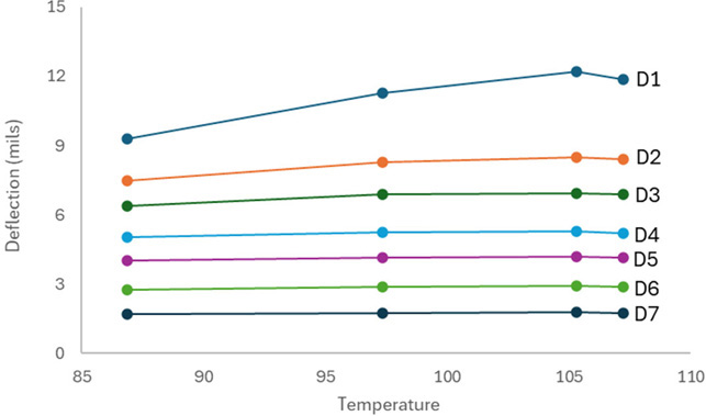
Numerous studies have used in situ testing to quantify the effects of temperature on pavement deflection (Kim et al. 1995, Lukanen et al. 2000, Ceylan et al. 2013, Zheng et al. 2019, Haider et al. 2021). Most of these studies tested deflection over a brief period (i.e., same day) to ensure that only temperature varied. Ramos-García and Castro (2011) measured pavement deflections at different times in a single day to relate changes in measured deflection with changes in pavement temperature. The first deflection pass was conducted early in the day, when the pavement surface was cooler, and the last deflection pass was conducted late in the day when the pavement surface had warmed. As shown in Figure 4, deflection measurements, conducted at the same location multiple times in a single day, increased as the temperature at the time of testing increased.
Asphalt materials are also viscoelastic; therefore, modulus values are dependent on temperature and loading time (or frequency). Kim (2008) indicated the elastic-viscoelastic correspondence principle can be used to account for the asphalt materials’ viscoelastic properties. Solatifar et al. (2019) and Kim et al. (2021) backcalculated the time-dependent dynamic modulus (E*) using FWD time history data.
Environmental Effects on Unbound Materials
Resilient modulus for unbound layers and subgrade soils is a function of density, applied stress, and moisture content, and is assumed to be independent of temperature. Although unbound layer density may vary over time, for pavement design purposes it is typically assumed to be constant.
The effect of the stress state on the unbound layer resilient modulus is determined using a universal constitutive equation as a function of bulk stress, octahedral shear stress, and atmospheric pressure. In the PMED software, this effect is only accounted for using Level 1 (i.e., laboratory or FWD testing) inputs for asphalt pavement designs. Moisture and temperature effects on resilient modulus values are considered for all input levels using a composite environmental adjustment factor. The EICM determines soil moisture, suction, and temperature as a function of time. The environmental adjustment factor is based on (NCHRP 2004):
| (Eq. 1) |
where,
| MR = | resilient modulus |
| Fenv = | environmental adjustment factor |
| MRopt = | resilient modulus at optimum conditions at any state of stress (assumes an independent variation with stress and moisture, density, and freeze/thaw conditions) |
If all other conditions are considered equal, as moisture content increases, layer moduli decrease, resulting in increased pavement deflections. While this can be expected for most fine-grained soils, it can also occur with coarse-grained materials, depending on the percentage of fine-grained material. In this regard, moisture can affect (1) the state of stress, through suction or pore water pressure, and (2) the soil structure, by damaging the interconnection of soil particles (Gaspard et al. 2020).
In frozen conditions, the resilient modulus of soils containing moisture can be 20 to 120 times greater than in unfrozen conditions. The presence of frost-susceptible soils, moisture, and subfreezing temperature can lead to ice lens development, potentially creating zones of differential roadway profile changes, and reduced strength during thawing conditions (Figure 5).
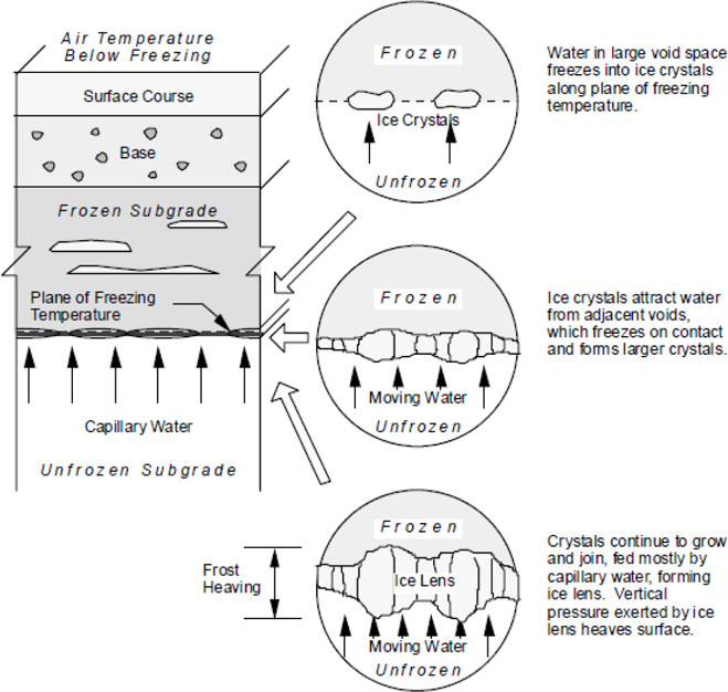
Figure 5. Ice lens development.
Hossain et al. (2000) investigated seasonal variation in subgrade soil properties and behavior due to temperature and moisture changes. The subgrade soil moduli were backcalculated using layered elastic theory. The study found most sites evaluated experienced relatively constant moisture conditions from season to season, with a moisture content change of 3 to 6 percent. Temperature and moisture effects on backcalculated layer moduli include the following (Long et al. 1997, Hossain et al. 2000, Chatti et al. 2017, and Muslim and Haider 2021):
- Higher surface temperatures resulted in lower backcalculated subgrade moduli.
- In most instances, seasonal changes had a greater effect on layer moduli than site variability. However, once deflections and moduli were temperature-corrected, seasonal and site variabilities were approximately equal.
- Temperature varied more than any other measured seasonal change. FWD testing at temperature extremes resulted in large variations in deflection and, therefore, the backcalculated subgrade moduli. To minimize this impact, the authors recommended conducting FWD testing at moderate temperatures (68°F to 104°F).
Environmental Effects on JPCP Slabs
The temperature gradient is the difference in temperature between the top and the bottom of a concrete slab. Temperature gradient plays a significant role in the daily curl of a concrete slab. During the warming period of the day, the top of the slab is warmer than at the bottom, and the difference in thermal expansion causes the slab to curl downward. In contrast, during the cooling period of the day, the bottom of the concrete slab is warmer than the top, which causes the slab to curl upwards Figure 6). Figure 6 represents the direction of influence, in practice the direction of curling often does not reverse.
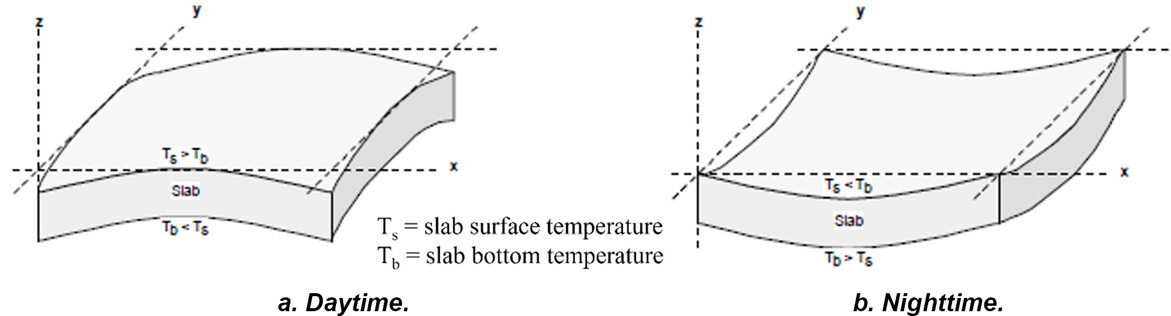
Figure 6. Slab curling.
Siddique et al. (2005) indicated the degree of curling and warping increased as the temperature gradient increased. Slab curling and warping can result in a loss of support at the slab corners and slab center, and when combined with the weight of the slab and traffic loading, can contribute to cracking or slab failure (Choubane and Tia 1995, Jeong and Zollinger 2004, Siddique et al. 2005).
A moisture gradient can also result in JPCP slab volume changes and cause curling and warping (Harr 1958, Mohamed and Hansen 1997, Belshe et al. 2011). Typically, the top of the JPCP slab is partially saturated while the bottom is close to saturation, which can result in cracking, especially when combined with a negative (daytime) temperature gradient.
Other JPCP moisture-related conditions include built-in curl and early-age shrinkage. These can cause the slab to permanently curl upward, leading to premature faulting and cracking (Siddique et al. 2005, Asbahan and Vandenbossche 2011, Nassiri and Vandenbossche 2011).
Effects of Freeze-Thaw
The resilient modulus of coarse- and fine-grained soils can be significantly impacted by freezing and thawing (Lee et al. 1995, Wang et al. 2017, Ishikawa et al. 2019). For frozen soils, the resilient modulus is a function of the moisture content. Upon thawing, the resilient modulus is significantly reduced; it gradually increases with moisture drainage during the recovery period. In general, stress dependency in the frozen soil was found to be negligible compared to the effects of temperature (Richter 2006).
To further describe this effect, Cole et al. (1981) obtained core samples and conducted laboratory resilient modulus testing of a sand material in frozen, thawed, and recovered conditions. Under frozen conditions, the resilient modulus of the sand material was approximately 14,500 psi (depending on the applied deviator stress) over a temperature range of about 15°F to 25°F. As the temperature increased to 32°F, the resilient modulus decreased rapidly to approximately 1,450 psi. Under thawed conditions, the resilient modulus ranged (with stress and moisture tension levels) from 5,800 to 29,000 psi.
Ovik et al. (2000) quantified the relationship between climatic factors, subsurface conditions, and pavement material properties for asphalt pavements in Minnesota. Variations in backcalculated layer moduli were used to define climate seasons. Unbound layer moduli were highest during frozen conditions and lowest during thawed conditions prior to moisture removal. In addition:
- Maximum layer moduli occurred from late November to February.
- Minimum layer moduli occurred during March.
- Subgrade modulus decreased during thawing from April to May. During this same time, base layer moduli were in the initial stages of recovery.
- Asphalt layer modulus was lowest from June to August.
Estimating Climatic Condition
Several models have been developed to quantify the impacts of climate conditions on material properties. The following sections summarize these models.
Pavement Temperature
Temperature profile models typically include statistics- or heat transfer-based models (Alland et el. 2018). Asphalt pavements are normally modeled using statistics-based models since the maximum temperature is more important than the temperature gradient, while concrete pavements are typically characterized using heat transfer-based modules (Lukanen et al. 2000).
AASHTO Asphalt Mix Effective Temperature
The AASHTO 1993 Guide recommends the effective temperature of the asphalt layer be determined using the mean temperature values from the near-surface, the mid-layer, and the bottom of the asphalt layer. The asphalt mix temperature is either directly measured or estimated from the sum of the measured surface temperature and the average air temperature over the previous five-day period.
Kim et al. (1995) noted that asphalt surface temperatures, measured at noon and late afternoon at one section, were essentially the same; however, the mid-depth temperatures differed by 45°F. When using the AASHTO 1993 Guide’s effective temperature method for FWD testing, the asphalt mix temperature becomes a function of only the pavement surface temperature, since the mean air temperature for the previous 5 days remains the same.
Superpave Temperature Estimation for Binder Selection
The Superpave binder selection procedure is based on the lowest air temperature and the highest seven-day average air temperature (Mohseni 1998). The seasonal asphalt pavement temperature monthly low and high-temperature data were used to develop the following models:
| (Eq. 2) | |
| (Eq. 3) |
where,
| Tpav-L = | low asphalt pavement temperature below the surface (°C) |
| Tpav-H = | high asphalt pavement temperature below the surface (°C) |
| Tair-L = | low air temperature (°C) |
| Tair-H = | high air temperature (°C) |
| Lat = | latitude of the section (degrees) |
| H = | depth of surface (mm) |
BELLS Model for Asphalt Pavements
Lukanen et al. (2000) used temperature data from the LTPP SMP to develop a model for estimating subsurface asphalt mix temperatures for deflection testing (referred to as the BELLS model). The BELLS model is used to estimate asphalt pavement temperature at a specified depth, using surface temperature, average air temperature 1 day prior to FWD testing, and time of day. Lukanen et al. (2000) noted the rate of surface cooling in shaded areas was significant. Therefore, two regression models were developed: BELLS2 for LTPP testing protocols and BELLS3 for the shade-adjusted surface temperatures.
| (Eq. 4) |
| (Eq. 5) |
where,
| Td = | pavement temperature at depth d (°C) |
| IR = | infrared surface temperature (°C) |
| d = | depth at which material temperature is to be predicted (mm) |
| T1-d = | average air temperature the day before testing (°C) |
| kr18 = | time of day, in a 24-hr clock system, but calculated using an 18-hr asphalt mix temperature rise- and fall-time cycle. |
Concrete Pavement Finite Difference Method
McCullough and Rasmussen (1999) developed the High PERformance Concrete PAVing software (HIPERPAV®) to estimate concrete temperature immediately after placement. HIPERPAV considers heat conduction from curing compounds and the heat of cement hydration. HIPERPAV incorporated the use of a 1D finite element technique; however, this required significant computational time to complete long-term analysis. In 2006, Ruiz et al. developed HIPERPAV II based on the 95th percentile values from a solar radiation database. In addition, Ruiz et al. (2006) replaced the 1D finite element procedure with a finite difference method (FDM) for the prediction of early-age and long-term concrete temperature.
Alland (2019) used two data sources, the Automated Surface Observation System and the Modern-Era Retrospective Analysis for Research and Applications Version 2 (MERRA2), to develop a method for predicting the pavement temperature profile. The weather dataset has information on shortwave radiation at the ground level, ambient temperature, wind speed, relative humidity, and cloud cover. Heat transfer through the pavement structure was calculated using the FDM. The models developed by Alland (2019) recognize the effect climate has on the pavement temperature profile prior to and during FWD testing.
Bentz (2000) developed a 1D finite difference scheme to predict the temperature and time of wetness for concrete pavements using heat transfer due to conduction, convection, and radiation.
Nonlinear Thermal Gradient Model for Concrete Pavements
Mohamed and Hansen (1997) developed a nonlinear model to determine an equivalent linear gradient through the concrete slab depth. The Mohamad and Hansen (1997) model was developed to produce the same curvature as the Westergaard (1926) linear-gradient solution. The Mohamed and Hansen (1997) model includes:
| (Eq. 6) |
where,
| ΔTeq = | equivalent linear temperature gradient (°C) |
| h = | slab thickness (m) |
| a = | concrete coefficient of thermal expansion (CTE) (m/m/°C) |
| M* = | constant dependent on the temperature distribution |
| (Eq. 7) |
| z = | distance from slab midplane (m); z is positive downward |
| ε(z) = | strain profile (m/m) |
Seasonal Variation
Annual seasonal variation can impact the properties of pavement materials, specifically layer stiffness and strength, and response to traffic loading. Seasonal variation impacts include changes in water table depth, freezing and thawing extent and duration, and moisture content variations.
Ksaibati et al. (2000) studied several locations on the Florida highway system to evaluate the change in base and subgrade layers moduli due to the proximity of the water table. FWD testing results showed a magnifying effect on the backcalculated base and subgrade modulus dependent on its moisture content.
Hanek (2000) and Janoo and Sheppard (2000) conducted studies to determine the impact of moisture content, during spring thaw, on backcalculated layer moduli in Montana. During thawing conditions, the moisture sensors showed a large and sudden increase in moisture content compared to measurements before freezing. Once thawing was completed, the moisture sensors detected an equally rapid decrease in moisture content (Hanek 2000). Janoo and Sheppard (2000) found similar behavior and determined thaw weakening initiated when the temperature dropped below 32°F.
Enhanced Integrated Climate Model
The EICM is a 1D coupled heat-and-moisture flow program for predicting temperature and moisture in the pavement structure (Lytton et al. 1993). The EICM uses project location, pavement material properties, and historical climatic data to generate weather patterns for rainfall, solar radiation, air temperature, cloud cover, wind speed, and snowfall throughout the year (Ruiz 2006). The EICM predicts the thermal gradient, temperature, pore water pressure, water content, frost heave, and drainage performance at various stages during the year. The EICM needs several inputs and includes (Table 1):
- The precipitation (Precip.) model generates precipitation patterns using data from the National Oceanic and Atmospheric Administration (Liang and Lytton 1989).
- The infiltration-drainage model determines the water infiltration through surface cracks and subsequent flow in the drainage layer (Liu and Lytton, 1985).
- The frost heave and thaw settlement model predicts the frost and thaw penetration, heave, and settlement in subgrade soils (Guymon et al. 1986).
- The climate-materials-structure model is a one-dimensional, forward finite difference, heat transfer model that estimates the frost penetration and temperature distribution (Dempsey et al. 1985). Base and subbase moduli are determined using unfrozen and frozen temperatures.
Table 1. Summary EICM Inputs (NCHRP 2004)
| Input | Description | PMED Use |
|---|---|---|
| Base/subgrade construction | Month and year |
|
| Existing pavement construction | Month and year |
|
| Pavement construction | Month and year |
|
| Traffic opening | Month and year |
|
| Type of design | New or rehabilitation |
|
| Weather-related hourly data | Air temperature |
|
| Precipitation |
| |
| Wind speed |
| |
| Percent sunshine |
| |
| Relative humidity |
|
A schematic of the EICM process is shown in Figure 7.
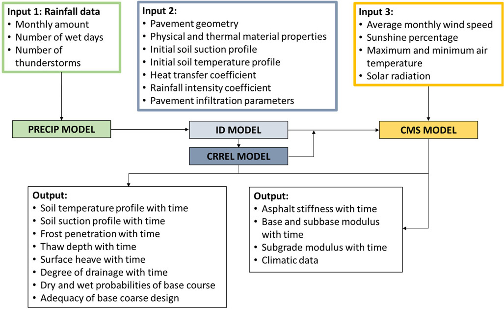
Within PMED, the EICM results are used with the material characterization, structural response, and performance prediction modules (NCHRP 2004). The general approach used to incorporate the EICM into PMED is shown in Figure 8.

External outputs, including a brief description and use within PMED, are summarized in Table 2.
Table 2. Summary EICM Outputs (NCHRP 2004)
| Output | Description | PMED Use |
|---|---|---|
| Unbound material resilient modulus adjustment factor | Determined from FF, FR, or FU, for every sublayer (defined by EICM)1 | Resilient modulus as a function of position and time |
| Temperature at the surface and midpoint of each asphalt bound sublayer | Mean, standard deviation, and quintile points for every analysis period (1 month or 2 weeks) | Fatigue and rutting prediction models |
| Hourly surface temperature | Every inch within bound layers | Thermal cracking prediction model |
| Volumetric moisture content of unbound layers | Average value of each sublayer | Rutting prediction model |
| Concrete layer temperature profile | Hourly | Cracking and faulting prediction model for JPCP and punchout prediction model for CRCP |
| Freeze-thaw cycles and FI | Annually | JPCP performance |
| Relative humidity | Monthly | Moisture gradients in JPCP and CRCP |
1 FF = adjustment factor for frozen condition; FR = adjustment factor for recovering conditions; and FU = adjustment factor for unfrozen condition.
Subgrade Moisture Model for Asphalt Pavements
Lytton et al. (1993) developed a method to predict the average monthly moisture content using site-specific climate, soil data, and roadway geometry. The Lytton et al. (1993) approach incorporates the following to determine subgrade moisture:
- Percent passing the No. 200 sieve
- Saturation water content
- Plastic limit
- Liquid limit
- Plasticity index
- Difference in water content between the plastic limit and saturation
- Suction at the plastic limit
- Monthly rainfall
- Specific gravity of solids
- Presence of paved shoulders
- Thornthwaite Moisture Index (TMI)
The TMI correlates rainfall and the water loss potential due to evaporation and transpiration and is calculated using the following equation (Thornthwaite 1948):
| (Eq. 8) |
where,
| TMI = | Thornthwaite Moisture Index |
| Ih = | Humidity Index |
| (Eq. 9) |
| Ia = | Aridity Index |
| (Eq. 10) |
| R = |
moisture surplus (runoff) – excess precipitation of potential evapotranspiration which occurs when soil is at the field capacity |
| D = |
moisture deficit – additional water required to create the potential evapotranspiration when the precipitation is insufficient |
| (Eq. 11) |
| (Eq. 12) |
| t = | temperature (°C) |
| I = | annual heat index in a particular year, a summation of monthly heat index values (i) |
| (Eq. 13) |
| d = | number of hours between sunrise and sunset in a month |
| N = | number of days for a given month |
High rainfall totals do not imply high TMI values since moisture loss may occur before it is absorbed into the soil. A series of calculations are used to determine the average monthly moisture content (Lytton et al. 1993).
Temperature Adjustment of FWD Measurements
Significant efforts have been undertaken to apply temperature corrections to FWD deflections, deflection basin parameters, and backcalculated layer moduli for asphalt pavements. The following summarizes methods for temperature adjustment of FWD measurements.
Adjustment of Deflection and Deflection Basin Factors
Cumberledge et al. (1974) studied the influence of subgrade moisture conditions on surface deflections. A multi-linear regression model was developed to quantify the changes in pavement surface temperature and subgrade moisture.
| (Eq. 14) |
where,
| Δδ60F = | change in surface deflection (mils) at a surface temperature of 60°F |
| ΔMC = | change in moisture content |
| %200 = | percent passing No. 200 sieve |
| Dp = | entire pavement thickness (in.) |
| LL = | Liquid Limit |
| γd = | density (lb/ft3) |
The Asphalt Institute (1982) temperature adjustment factor is a function of the measured pavement temperature at the time of deflection testing and the untreated base layer thickness (Figure 9). The temperature adjustment factor normalizes the measured deflection to a standard temperature of 20°C.
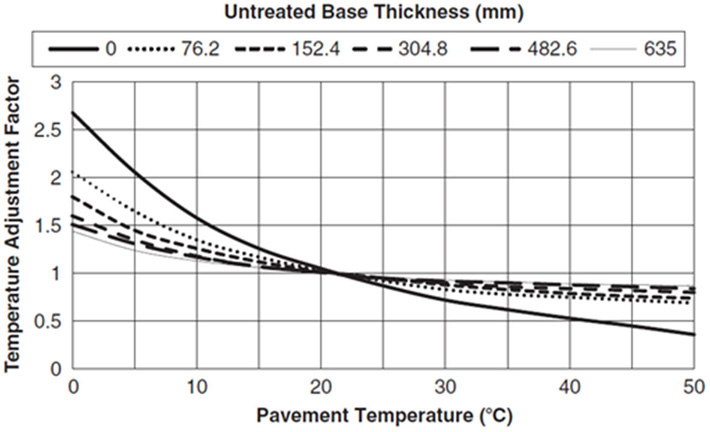
Figure 9. Asphalt Institute temperature adjustment factor.
The AASHTO 1993 Guide uses generated curves to correct the measured center deflection to a standard temperature of 68°F using the following equation:
| (Eq. 15) |
where,
| do = | deflection measured at the center of the load plate and adjusted to 68°F (in.) |
| p = | applied load (psi) |
| a = | load plate radius (in.) |
| D = | total thickness of pavement layers above subgrade (in.) |
| MR = | resilient modulus (psi) |
| Ep = | effective modulus of all layers above the subgrade (psi) |
Figure 10 illustrates the adjustment factors for asphalt pavements on granular and asphalt stabilized bases and cement and pozzolanic bases.
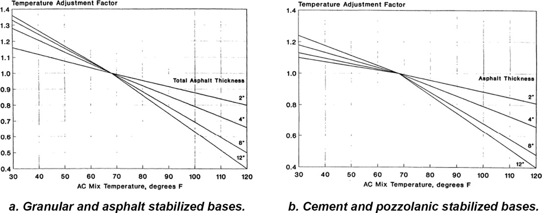
Figure 10. Center deflection temperature adjustment factors.
Adjustment factors were developed from a limited number of sites and the AASHTO 1993 Guide recommends development of agency-specific temperature factors. Johnson and Baus (1992) noted the inaccuracy of the AASHTO 1993 Guide adjustment factors, especially at surface temperatures greater than 100°F.
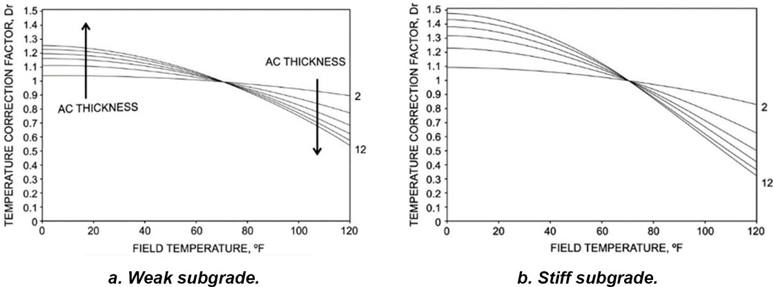
The Strategic Highway Research Program (SHRP) used Boussinesq’s one-layer deflection equation to correct the maximum deflection due to temperature variation (SHRP 1993). Two charts were developed for asphalt pavements, one for weak subgrades and the other for stiff subgrades, emphasizing the importance of the subgrade in deflection adjustment (Figure 11).
The temperature adjustment factor developed by an FWD equipment manufacturer corrects the measured deflection to a reference temperature of 20°C as a function of asphalt layer thickness and an applied load of 50 kN (Dynatest 1995).
| (Eq. 16) |
where,
| kT = | temperature adjustment factor |
| Td = | mean asphalt pavement temperature (°C) |
| ha/b = | thickness of asphalt pavement layer (mm) |
Kim et al. (1995) proposed a model to correct the maximum surface deflection to a reference temperature of 68°F. This procedure was developed based on deflection measurement and the mid-depth temperature of the asphalt layer.
| (Eq. 17) |
where,
| d68 = | adjusted deflection to a reference temperature of 68°F (mil) |
| dT = | deflection measured at temperature T (mil) |
| α = | 3.67 × 10⁻⁴ × t1.4635 for wheel paths |
| = | 3.65 × 10⁻⁴ × t1.4241 for lane centers |
| t = | thickness of the asphalt layer (in.) |
| T = | asphalt layer mid-depth temperature (°F) |
Park et al. (2002) further expanded the work by Kim et al. (1995) by using multi-load-level deflections and pavement temperatures to apply temperature correction at variable offset distances. Park et al. (2002) also determined the FWD load level does not affect the temperature dependence of the measured deflection; therefore, the correction factors can be used for different load levels.
Lukanen et al. (2000) evaluated temperature-dependent deflection basin shape factors. Asphalt pavement basin shape factors vary with asphalt temperature and are influenced by a variety of other factors such as asphalt temperature and layer thickness, stiffness and thickness of the pavement structure, subgrade stiffness, depth to the apparent stiff layer (i.e., bedrock), and deflection offset. A summary of deflection and basin shape factors includes:
- AREA value is the ratio of the pavement deflection to the deflection at the center of the load. The AREA value is calculated as:
(Eq. 18) where,
A = AREA value (unitless) D0 = deflection at center of the applied load D1 = deflection at 12 in. from the applied load D2 = deflection at 24 in. from the applied load D3 = deflection at 36 in. from the applied load - F1 shape factor is the curvature of the deflection basin. The F1 shape factor is inversely proportional to the ratio of the pavement stiffness to the subgrade stiffness:
(Eq. 19) where,
F1 = shape factor D0 = deflection at center of the applied load D1 = deflection at 12 in. from the applied load D2 = deflection at 24 in. from the applied load - Surface Curvature Index is the difference between the deflection at the center of the load and the deflection at 12 in.
Dawson et al. (2016) determined that pavement temperatures have a greater impact on deflections closer (within 12 in.) to the applied load than on deflections at a greater distance (24 in. or greater). The following equation was developed for temperatures between 0°C and 50°C.
| (Eq. 20) |
where,
| APDi = | average peak pavement deflection at sensor i |
| ωi and Ci = | regression constants for sensor i |
The resulting temperature adjustment factor (normalized to a standard temperature of 21°C) equation includes:
| (Eq. 21) |
where,
| TAF = | temperature adjustment factor |
| A, B, C = | regression constants |
| T = | measured pavement surface temperature (°C) |
Pais et al. (2020) developed a temperature adjustment model based on the asphalt layer thickness, subgrade stiffness, distance between sensors, applied load, and pavement temperature at the time of FWD testing.
| (Eq. 22) |
where,
| DR = | deflection ratio (deflection at 20°C dived by the deflection at temperature T) |
| T = | temperature (°C) |
| ßi = | statistical coefficients |
| d = | distance (m) |
| H = | asphalt layer thickness (m) |
| E = | subgrade stiffness (megapascals [MPa]) |
Correcting Moduli to Reference Temperature
Kim et al. (1995) proposed the following equation for correcting backcalculated asphalt layer moduli to a reference temperature:
| (Eq. 23) |
where,
| E68 = | adjusted asphalt layer modulus to a reference temperature of 68°F (psi) |
| ET = | backcalculated asphalt layer modulus (psi) at temperature T (°F) |
| T = | asphalt layer mid-depth temperature at the time of FWD testing (°F) |
The Chen et al. (2016) equation for adjusting the asphalt layer moduli to a reference temperature of 77°F included:
| (Eq. 24) |
where,
| E77 = | adjusted asphalt layer modulus to a reference temperature of 77°F |
| ET = | backcalculated asphalt layer modulus (psi) at temperature T (°F) |
| T = | asphalt layer mid-depth temperature (°F) at the time of FWD testing |
Lukanen et al. (2000) developed the following temperature adjustment model using backcalculated asphalt moduli from more than 40 LTPP sections.
| (Eq. 25) |
where,
| ATAF = | asphalt temperature adjustment factor |
| slope = | slope of the log modulus versus temperature equation (1/degrees °C) |
| = | -0.0195 for wheel path locations |
| = | -0.021 for mid-lane locations |
| Tr = | reference mid-depth asphalt layer temperature (°C) |
| Tm = | mid-depth asphalt layer temperature at the time of measurement (°C) |
Most of the slopes for the Lukanen et al. (2000) model ranged from -0.010 to -0.027. The slope correlates with the latitude of the section and the asphalt binder grade. The variation in intercept and slope from station to station was caused by factors including asphalt binder and mix characteristics, pavement structural variations, surface condition, and asphalt thickness (Lukanen et al. 2000).
Using the Modulus program, Chen et al. (2000) developed an asphalt layer modulus temperature correction model. Chen et al. (2000) showed that deflections at radial distances of 0 and 8 in. were affected by temperature, while deflections further from the load remained almost constant at various temperatures (model based on asphalt layer thicknesses greater than 3 in.).
| (Eq. 26) |
where,
| ETW = | adjusted modulus at Tw (MPa) |
| ETC = | backcalculated modulus at Tc (MPa) |
| Tc = | mid-depth asphalt mix temperature measured during FWD test (°C) |
| TW = | reference temperature (defined as 25°C) |
Seasonal Adjustment of FWD Measurements
The AASHTO 1993 Guide was the first widely used pavement design method to consider site-specific seasonal variations of the subgrade modulus. Two methods are recommended for assessing the impact of moisture content on resilient modulus (AASHTO 1993):
- Conduct laboratory testing to determine the relationship between moisture content and resilient modulus. In situ moisture content can be used to estimate the resilient modulus during each season.
- Conduct FWD testing during various seasons and backcalculate the representative resilient modulus for each season.
The seasonal data is used to determine an effective modulus. The effective modulus is a weighted value of equivalent annual damage for each independent climate season (AASHTO 1993). The seasonal moduli are used to estimate the relative damage. The relative damage and average annual relative damage are calculated using:
| (Eq. 27) |
| (Eq. 28) |
where,
| ut = | relative damage per season |
| ūt = | average annual relative damage |
| MR = | measured resilient modulus per month (psi) |
| n = | number of measurements |
Figure 12 illustrates an example of the AASHTO 1993 Guide nomograph solution for determining the relative damage.
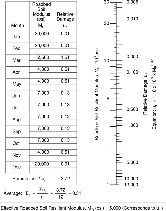
Figure 12. Example calculation of effective modulus for asphalt pavements.
The AASHTO 1993 Guide does not explicitly consider seasonal variation in asphalt overlays. The method is based on limited knowledge of subgrade modulus variation, and how the variation may differ according to project location, material type, and other factors (Richter 2006).
Typically, granular soils vary with changes in bulk stress, while fine-grained soils vary primarily as a function of applied deviator stress (Richter 2006). The following model predicts changes in modulus as a function of changes in moisture (NCHRP 2004):
| (Eq. 29) |
where,
| MR = | resilient modulus at a given time (psi) |
| MRopt = | resilient modulus at a reference condition (psi) |
| a = | minimum log (MR/MRop) (see Table 3) |
| b = | maximum log (MR/MRopt) (see Table 3) |
| km = | regression parameter (see Table 3) |
| (S – Sopt) = | variation in the degree of saturation expressed in decimal |
Table 3. ME Model Coefficients for Coarse- and Fine-Grained Materials (NCHRP 2004)
| Parameter | Coarse-Grained | Fine-Grained |
|---|---|---|
| a | -0.3123 | -0.5934 |
| b1 | 0.3 | 0.4 |
| km | 6.8157 | 6.1324 |
1Conservatively assumed, corresponds to modulus ratios of 2.0 (coarse-grained) and 2.5 (fine-grained).
The resilient modulus, at or near the optimum moisture content and the maximum dry density, is estimated using a generalized constitutive model. The nonlinear elastic coefficients and exponents of the model are determined using linear or nonlinear regressions to fit the model to laboratory-determined resilient moduli. The generalized model includes:
| (Eq. 30) |
where,
| MRopt = | resilient modulus at a reference condition (psi) |
| k1-3 = | regression constants |
| Pa = | atmospheric pressure |
| θ = | bulk stress |
| τoct = | octahedral shear stress |
In the Asphalt Institute’s procedure, seasonal variations are considered using the mean annual air temperatures (MAAT) of 45°F, 60°F, and 75°F (Asphalt Institute 1982). Separate asphalt pavement design charts were developed for each temperature MAAT. The design charts for MAAT of 45°F and 60°F were developed by varying the subgrade modulus and the k1 coefficient (MR = k1θk2) for the granular base layer to reflect freezing, thawing, and recovery conditions, while the asphalt layer moduli were varied by mean monthly temperature (Asphalt Institute 1982). The resulting subgrade soil and granular base moduli are summarized in Table 4 and Table 5, respectively.
Table 4. Subgrade Moduli for Asphalt Institute Method (adapted from Asphalt Institute 1982)
| MAAT (°F) | Subgrade Modulus (ksi) | |||||||||||
|---|---|---|---|---|---|---|---|---|---|---|---|---|
| Dec | Jan | Feb | Mar | Apr | May | Jun | July | Aug | Sep | Oct | Nov | |
| 45 | 4.5 | 15.9 | 27.3 | 38.7 | 50.0 | 0.9 | 1.6 | 2.3 | 3.1 | 3.8 | 4.5 | 4.5 |
| 12.0 | 21.5 | 31.0 | 40.5 | 50.0 | 6.0 | 7.2 | 8.4 | 9.6 | 10.8 | 12.0 | 12.0 | |
| 22.5 | 29.4 | 36.3 | 43.1 | 50.0 | 15.8 | 17.1 | 18.5 | 19.8 | 21.2 | 22.5 | 22.5 | |
| 60 | 4.5 | 4.5 | 27.3 | 5.0 | 1.4 | 2.1 | 2.9 | 3.7 | 4.5 | 4.5 | 4.5 | 4.5 |
| 12.0 | 12.0 | 31.0 | 50.0 | 7.2 | 8.4 | 9.6 | 10.8 | 12.0 | 12.0 | 12.0 | 12.0 | |
| 22.5 | 22.5 | 38.3 | 50.0 | 18.0 | 19.1 | 20.3 | 21.4 | 22.5 | 22.5 | 22.5 | 2.5 | |
Table 5. Monthly Granular Base k1 Values (adapted from Asphalt Institute 1982)
| MAAT (°F) | Monthly Value for k1 (psi) | |||||||||||
|---|---|---|---|---|---|---|---|---|---|---|---|---|
| Dec | Jan | Feb | Mar | Apr | May | Jun | July | Aug | Sep | Oct | Nov | |
| 45 | 8.0 | 12.0 | 16.0 | 20.0 | 24.0 | 2.0 | 3.2 | 4.4 | 5.6 | 6.8 | 8.0 | 8.0 |
| 12.0 | 18.0 | 24.0 | 30.0 | 36.0 | 3.0 | 4.8 | 6.6 | 8.4 | 10.2 | 12.0 | 12.0 | |
| 60 | 8.0 | 16.0 | 24.0 | 2.0 | 3.5 | 5.0 | 6.5 | 8.0 | 8.0 | 8.0 | 8.0 | 8.0 |
| 12.0 | 24.0 | 36.0 | 3.0 | 5.3 | 7.5 | 9.75 | 12.0 | 12.0 | 12.0 | 12.0 | 12.0 | |
Temporal and Diurnal Variations of Longitudinal Profile Measurements
The temporal and diurnal temperature and moisture variations can significantly influence pavement layer material properties and contribute to variation in longitudinal profiles (Ovik et al. 2000). Several aspects of the pavement surface shape make measuring longitudinal profiles related to environmental variables (i.e., temperature and moisture) challenging. These include (Karamihas et al. 1999):
- Combined, the lateral position, and temporal and diurnal variations in profile are only a sample of the roadway shape.
- Lateral position of measurement strongly influences the longitudinal profile.
- Roughness variations of 10 percent, over a 24-hour period, are common with concrete pavements.
Several studies showed daily temperature variations of longitudinal profile measurements can significantly influence the computed IRI (Novak and DeFrain 1992, Karamihas 1999, Karamihas and Senn 2012). For asphalt pavements, the temporal and diurnal temperature changes can accelerate distress progression (e.g., rutting, thermal cracking, top-down cracking, bottom-up cracking, and IRI). For concrete pavements, the effect of temperature changes can be more pronounced due to slab curling and warping (Chang et al. 2008, 2010, Karamihas and Senn 2012). As noted previously, high-temperature gradients can result in differential volume changes, which in turn result in curling and warping, negatively impacting ride quality and potentially increasing slab cracking.
Asphalt Pavements
Novak and Defrain (1992) investigated the effects of seasonal variation of longitudinal profile measurements on asphalt pavements in Michigan. The study found pavements subject to frost action are rougher in the winter and smoother in the summer and opposite of pavements not exposed to frost action, where they tend to be rougher in the summer than in the winter. The study also illustrated how a longitudinal profile can be used to evaluate the cause of deterioration, and aid in the selection of maintenance, rehabilitation, and reconstruction treatments for improving ride quality.
Several studies found that depression, swelling, and frost heaving significantly contributed to increased pavement surface roughness (Novak and DeFrain 1992, Hassan et al. 1999, Ovik et al. 2000, Kameyama et al. 2002, and Drumm and Meier 2003). Bae et al. (2008) evaluated 34 asphalt sections using the LTPP SMP data and showed roughness deterioration occurred with increases in the magnitude and variation of moisture at nonfreezing locations and with variations in moisture at freezing locations. Bae et al. (2008) also found thinner pavement sections and subgrade soils with high percent fines contributed to accelerating roughness deterioration.
Shuichi et al. (2002) noted that pavements subjected to frost are rougher during winter months than during summer months. The study also noted that frost action can occur in cut sections when abundant moisture is present. In these instances, roughness was found to increase two to five times more during the winter than in any other season (Shuichi et al. 2002).
Lytton et al. (1976) quantified roughness on pavements with expansive clay subgrades as a function of dominant wavelength and roughness amplitude. The dominant wavelengths for swelling soils were in the range of 10 to 30 ft. On airfield pavements, Uzan et al. (1984) noted dominant wavelengths for expansion soils in the range of 16 to 33 ft. On non-expansive soils, roughness increased faster over short wavelengths than over longer wavelengths, whereas on expansive soils, the effect was reversed.
Concrete Pavements
Karamihas and Senn (2012) examined roughness and its progression on 21 LTPP SPS-2 sections in Arizona. The SPS-2 site included 12 sections from the standard LTPP experiment and nine supplemental sections added by the Arizona DOT. The investigation showed:
- Roughness increased with the progression of transverse and longitudinal cracking.
- Areas of localized roughness were caused by built-in defects.
- Curl and warp significantly contributed to roughness on many of the sections.
- Roughness did not steadily increase with time due to temporal and diurnal changes of slab curling and warping.
The 2GCI analysis is commonly used to quantify slab curling and warping. Algorithms are used to estimate the needed pseudo-strain gradient (PSG) to deform each slab into the shape present in the measured profile (Karamihas et al. 2023). The average PSG values are used to summarize the curl and warp within each measured longitudinal profile and, over time, the variation of the average PSG can be used to explain changes in JPCP roughness (Karamihas et al. 2023).
Chang et al. (2008) noted that JPCP roughness is a function of a curvature-related component (i.e., due to curling and warping) and a non-curvature-related component (i.e., due to pavement distresses). The daily changes in slab curvatures were analyzed in terms of PSG and demonstrated the effect on roughness (i.e., as PSG increases, slab curling increases) (Figure 13).
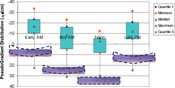
Chang et al. (2008) also found daily impacts on the Half-car Roughness Index (HRI) as high as 10 in/mi and an average of approximately 2.5 in/mi. This finding highlights the importance of specifying the time of day for longitudinal profile measurement, especially for agencies who use incentives and disincentives
in their construction specifications. The daily roughness impacts can also affect pavement management activities. Significant daily changes can result in large fluctuations in roughness, thereby impacting the prediction of preservation and rehabilitation treatment timing, and potentially treatment type selection.
Curl and Warp Measurement
Early studies used graphical plots of profilograph traces for quantifying JPCP curling and warping (Stanton 1944, Moyer 1950, Housel 1962, Tremper and Spellman 1963), while others used direct measurement of elevation changes [SHCK 1949, Evans and Drake 1959, Lowrie and Nowlen 1960, American Association of State Highway Officials (AASHO) 1962, Spellman et al. 1970, Armaghani et al. 1987, Poblete et al. 1988, Goldsberry 1998, Yu et al. 1998, Yu and Khazanovich 2001, Jeong and Zollinger 2004, Rao and Roesler 2005, Ardani 2006, Rao 2006]. Modern studies have quantified curling and warping using low-speed, inclinometer-based profilers operated along key locations (e.g., lane edge, wheel paths). Several studies measured longitudinal roughness and used IRI to express early-age behavior or changes at various times of day (Ceylan et al. 2007, Kim et al. 2007, Pradena and Houben 2017). Typically, curling and warping were quantified by the analysis of the measured profiles according to slab temperature at various depths and material strain.
Lederle et al. (2011) and Lederle (2011) quantified curling and warping from transverse profiles measured at the MnROAD research facility. The measured transverse profiles were associated with profiles predicted by a finite element program at different slab depth temperatures.
Ceylan et al. (2016) used light detection and ranging (LiDAR) systems measurements to quantify slab curling and warping of in-service pavements in Iowa. The LiDAR scans were used to develop 3-dimensional (3D) surface profiles for each test slab.
Several studies demonstrated the impact of curling and warping on longitudinal profile measurements using filtered elevation plots (Sayers and Karamihas 1996, Perera et al. 1998, Karamihas et al. 1999, Perera et al. 2005) and power spectral density plots (Perera and Kohn 1994, Karamihas et al. 2001). Others have attributed IRI changes to changes in curling and warping over temporal and diurnal cycles (Karamihas et al. 1999, Karamihas et al. 2001, Johnson et al. 2010).
Yang et al. (2018) described the use of 3D surface measurements from LiDAR to study the response of pavements to environmental factors. Slab deformation was characterized using elevation profiles along diagonals, which is not a current measurement of conventional high-speed profilers. Yang et al. (2018) noted project- or research-level investigations of slab deformation might benefit from measurements in 3D, rather than the wheel paths.
Yang (2019) conducted LiDAR field surveys of in-service JPCP. The 3D scans were used to study slab deflections due to curl and warp using the wavelet analysis. Yang et al. (2021) applied continuous and discrete wavelet transforms to JPCP profiles. The investigation studied the content within each pseudo-frequency range of raw profiles, profiles produced using slab-by-slab curve fits to the Westergaard model, and profiles filtered through the IRI algorithm.
Curl and Warp Characterization
Based on MnROAD data, Vandenbossche (2003) identified “geometric pavement slope and surface irregularities” from slab profiles. A second-order curve fit was used to approximate slab curvature.
| (Eq. 31) |
| (Eq. 32) |
where,
| y(x) = | displacement profile as a function of distance along the slab diagonal |
| A, B, C = | coefficients |
| K = | slab curvature |
| x = | location along the profile traverse |
| y = | measured displacement |
Observations for quantifying curling and warping using measured longitudinal profiles included (Vandenbossche 2003):
- Slab curvature, as a single parameter, was advantageous for comparing a range of temperature conditions between and within MnROAD cells.
- Predicting measured curvature depended on thermal loading, the radius of relative stiffness, and slab length.
- Curvature may vary within a given slab due to the influence of gravity and the presence of load transfer devices.
Wells et al. (2006) monitored doweled and undoweled slabs within 72 hours of placement. This study quantified slab curvature using the method described by Vandenbossche (2003) and the profile measured 1- ft from the slab edge. Asbahan and Vandenbossche (2011) conducted a 2-year evaluation of the same slabs to quantify the impacts of temperature and moisture gradients, and joint load transfer on slab deformation.
Chen et al. (2016) used a second-order curve fit approach for quantifying transverse profiles of an in-service JPCP. The deflection difference between the slab edge and the center of the slab was used to quantify slab deformation. Slab curvature was estimated using the second derivative.
Lederle et al. 2011 and Lederle 2011 proposed the following methods to process the profile measurements to remove the pavement cross slope and “extraneous points”:
- Polynomial Curvature Method: profiles were generated based on curvature versus distance across the slab derived from the fitted polynomial and compared to measured profiles.
- Ah Method: predicted profiles were generated using the difference between the slab midpoint and the edges and compared to measured profiles.
- Minimum Error Method: predicted profiles were generated by applying a polynomial curve fit to the measured profiles and compared to the measured profiles.
As noted previously, Ceylan et al. (2016) evaluated the degree of curling and warping using LiDAR data collected on four highway locations in Iowa. The LiDAR data was processed “for registration and segmentation” and fitted using a quadratic equation. The extent of curling and warping was determined longitudinally, transversely, and diagonally across the slab service.
Byrum Curvature Index
Byrum (2001a, b) demonstrated the use of a curvature index (CI) on profile measurements on JPCP and jointed reinforced concrete pavements from the LTPP GPS-3 and GPS-4, respectively. CI is defined as:
| (Eq. 33) |
where,
| CI = | curvature index |
| yn+i = | profile elevation at sample points |
| xn+i = | longitudinal distance at sample points |
Equation 33 can be further reduced to (Sayers and Karamihas 1998 and Hudson et al. 1985):
| (Eq. 34) |
where,
| CIn = | three-point estimate of curvature for the corresponding interval |
| Δx = | profile sample spacing |
| iΔx = | interval over which slope is calculated |
The overall CI is determined by summing the curvature estimates at 6 in., 24 in., and 48 in.
In 2006, Byrum applied a curvature variation threshold to identify the locations of joints and cracks. Profile measurements with high curvature values were identified as imperfections. The CI calculation excluded the profile measurements within 2 ft of the identified imperfections. This approach was also used to identify rocking, pumping, and faulting (Byrum 2006, 2010).
Curve Fitting
Sixbey et al. (2001) analyzed profile measurements of prematurely transverse cracked JPCP. Profile testing was conducted multiple times over a single day and the maximum deformation was used to determine individual slab curvature. A third-order fit was used to remove the linear trend from the fitted and measured profiles. From this analysis, the location of maximum deformation was found to occur where the difference between the measured and the fitted profile had the largest absolute value.
Fitting to an Assumed Slab Profile
Chang et al. (2007a) evaluated seasonal and diurnal changes on sections throughout the United States. Evaluation of diurnal changes was based on repeated profile measurements collected over a 24-hour period (early and mid-morning, and early and mid-afternoon) per season over a yearly cycle.
Chang et al. (2008) quantified curling and warping by fitting individual slab profiles to an assumed shape using the Westergaard equation. Individual slab profiles were isolated by locating narrow spikes representative of joint locations. Chang et al. (2008) used up to 10 repeat profile measurements (point laser at a 0.25 interval) at each site. Slab profiles were preprocessed by removing up to 2 in. of profile length at each end and any linear trends. A fitting procedure was used to find the best fit between the assumed slab shape and the measured profile and expressed in terms of PSG.
| (Eq. 35) |
where,
| z(x) = | fitted displacement profile |
| f = | defines the shape of the slab |
| x = | distance along with the slab with its origin at the slab center |
| b = | slab length |
| l = | radius of relative stiffness |
| z0 = | uplift at the slab ends in the fitted function |
| (Eq. 36) |
where,
| PSG = | “Pseudo-strain gradient” (strain per in. of depth), proportional to the magnitude of deformation |
| µ = | Poisson’s ratio |
| l = | radius of relative stiffness |
Chang et al. found a strong relationship between HRI and average PSG (2007a, 2008). The following summarizes studies conducted using the Chang et al. (2007a, 2008) method:
- Karamihas and Senn (2012). Assessed measured longitudinal profiles from the Arizona LTPP SPS-2 site. The analysis found the sections with lower-strength concrete and large diurnal and seasonal
- Ruiz et al. (2008). Examined changes and variations in PSG to assess premature cracking of an in-service JPCP. The assessment was conducted using longitudinal profile measurements tested in the morning and in the afternoon of the same day.
- Merritt et al. (2015). Investigated the potential presence of curling on an in-service JPCP. Diurnal longitudinal profile testing was conducted in February and August of the same year and confirmed the roughness was due to slab curling.
changes in IRI had a strong linear relationship between IRI and average PSG. The higher-strength concrete sections had minor changes in IRI.
Profile Decomposition
Siddique (2004) proposed using a Fast Fourier Transform to separate factors unrelated to curling and associating roughness to slab curl at partial (e.g., half, third) and full slab lengths. Curling was reported by comparing the reduction in the IRI without the curl components and the IRI of the original profile.
Gagarin et al. (2004) used the Hilbert-Huang Transform (HHT) to filter JPCP longitudinal profile measurements. Graphical plots were used to identify slab curling from other characteristics (e.g., texture, faulting).
Adu-Gyamfi et al. (2010) used the HHT tool to characterize roughness from measured longitudinal profiles. The HHT uses a profile decomposition to identify “intrinsic mode functions.” The intrinsic mode function shape is dependent on the properties of the measured signal and is best suited for quantifying signals with fluctuation severity changes or changes in the contributing frequencies.
Survey of State Highway Agencies
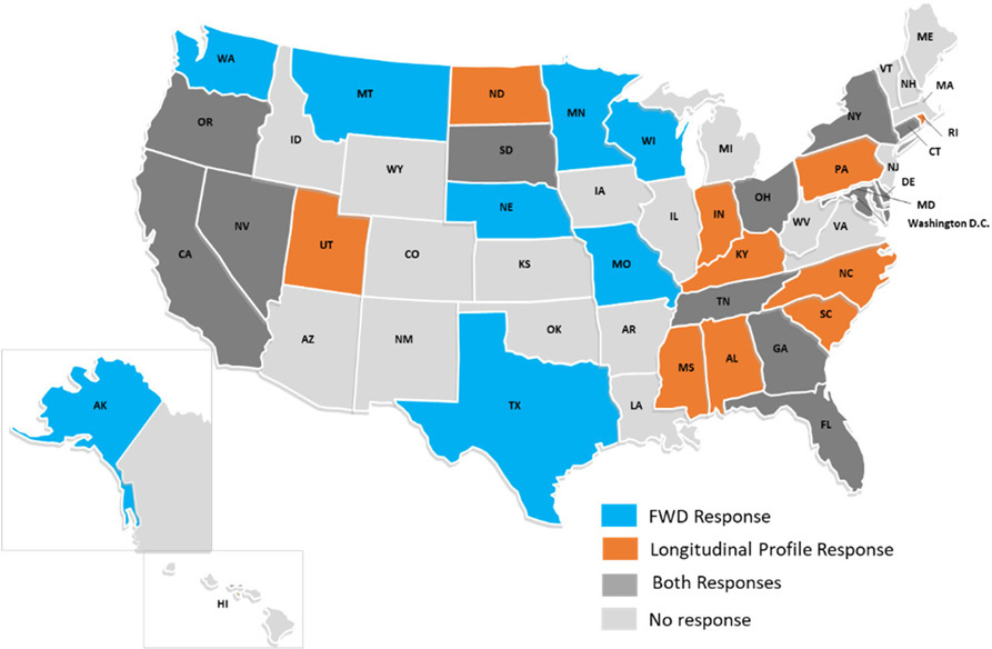
Two questionnaires were developed to identify agency practices related to temperature and moisture adjustments for FWD and longitudinal profile measurements. Both questionnaires were sent to all 50 SHAs, the District of Columbia, and Puerto Rico. One questionnaire was specific to FWD testing and was given to the pavement design engineer. The other was specific to longitudinal profile measurements and was given to the pavement management engineer. The questionnaires and agency responses are summarized in Appendix A.
In total, 20 agency representatives responded to the FWD questionnaire, and 21 agency representatives responded to the longitudinal profile questionnaire (Figure 14).
FWD Responses
Agencies were asked several questions related to FWD testing, temperature and moisture determination at the time of FWD testing, and challenges in adjusting FWD measurements to temperature and moisture conditions. The following summarizes the received responses:
- FWD testing:
- Three agencies indicated FWD testing was not conducted (not applicable).
- Thirteen agencies indicated FWD testing was conducted only at the project level.
- Four agencies indicated FWD testing was conducted at both the project and the network levels.
- None of the respondents indicated FWD testing was conducted at only the network level.
- Determining subsurface temperature:
- Thirteen agencies indicated subsurface temperatures were not measured.
- Four agencies indicated subsurface temperatures were measured (multiple responses).
- One agency indicated conducting field measurements.
- One agency used air temperature.
- Three agencies used prediction models to estimate subsurface temperatures.
- Three agencies did not respond to this question.
- Determining moisture conditions:
- None of the responding agencies determined subsurface moisture.
- Seasonal monitoring sites:
- None of the responding agencies conducted a SMP.
- Challenges with applying temperature and moisture adjustment (multiple responses):
- Nine agencies indicated limited availability of time.
- Nine agencies indicated uncertainty in how to use or apply the adjustments.
- Five agencies indicated budget constraints.
- Four agencies indicated adjustments were not needed.
Longitudinal Profile Responses
Like the FWD questionnaire, agencies were asked multiple questions related to profile measurements. The following provides a summary of responses:
- Profile testing:
- Twenty agencies indicated collecting profile measurements on the National Highway System (NHS).
- Sixteen agencies indicated collecting profile measurements on non-NHS roadways.
- Twenty agencies indicated collecting project-level measurements as part of construction ride specifications.
- Determining temperature and moisture conditions:
- None of the responding agencies indicated measuring temperature gradients and moisture profiles.
- None of the responding agencies indicated measuring JPCP slab curling and warping.
- Challenges with applying temperature and moisture adjustment (multiple responses):
- Fifteen agencies indicated being unsure how to use or apply adjustments.
- Seven agencies indicated having limited budget or limited time availability.
- Five agencies indicated temporal and diurnal adjustments to longitudinal profile were not needed.
The results of the agency surveys provided insight into the use and application of temporal and diurnal adjustments to FWD and longitudinal profile measurements by SHA’s. Although the questionnaire
response rate was low (less than 40 percent of SHAs), the response does support the need to summarize the reasons for applying temperature and moisture adjustments along with a viable and easy to use approach for making any needed adjustments.


