LTPP Data Analysis: Improving Use of FWD and Longitudinal Profile Measurements (2024)
Chapter: 4 Evaluation of Climatic Conditions
CHAPTER 4
Evaluation of Climatic Conditions
Definition of Seasons
A definition of season (i.e., spring, summer, fall, winter) was required to group the SMP climate data for analysis. The duration (months) of each season is typically defined as the change in the temperature cycles. For practical applications, seasons are typically set to have an equal duration (i.e., 3 months); however, seasonal changes can originate at various times each year and seasons can last more or less than 3 months depending on the location and climatic conditions. For example, the Minnesota DOT (MnDOT) defines five seasons using the three-day average temperature (TAVG), the thawing index (TI), and the FI (Table 12).
Table 12. MnDOT Season Definitions (adapted from Ovik et al. 1996)
| Season | Condition | Begins | Ends |
|---|---|---|---|
| Winter | Layers frozen | FI > 162°F-days | TI > 25°F-days |
| Early Spring | Base thaws | TI > 25°F-days | ~28 days layer |
| Late Spring | Base recovers | End of Season II | TAVG > 63°F |
| Summer | Higher temperatures, lower asphalt layer modulus | TAVG > 63°F | TAVG < 63°F |
| Fall | Standard season | TAVG < 63°F | FI > 162°F-days |
Climate data sources considered for the analysis included the PMED monthly climate summary file, generated as part of the output for each of the SMP sections, the LTPP Automatic Weather Station (AWS), and the Virtual Weather Station (VWS) tables. Due to the impact of moisture and frost penetration on layer moduli, precipitation, FI, and air temperature, were also taken into consideration.
Given a project location (i.e., longitude and latitude), PMED automatically selects several weather stations closest to the project and creates a VWS file (AASHTO 2020). The output file contains the monthly average values for a given climatic parameter over the project duration (Table 13). PMED only calculates an annual FI; however, sufficient data is available to calculate a seasonal FI.
Due to gaps in the data records the AWS weather information is limited compared to the VWS data. The VWS has significantly more points due to data acquisition from multiple OWSs (Operating Weather Stations). However, the selection of the OWS to form the statistical basis for a VWS is a critical consideration. Aspects such as the distance, elevation, terrain features, and temporal coverage between the OWS and VWS must be taken into consideration for the proper OWS selection.
Table 13. Climatic Data Sources
| Source | Inputs | |
|---|---|---|
| PMED |
|
|
| LTPP |
|
|
Schwartz et al. 2015 investigated the impact on pavement distress from different weather sources and concluded there were no systematic patterns in the discrepancies of PMED-predicted distresses using AWS versus MERRA versus VWS versus OWS weather data sources.
The daily air temperature and total precipitation values were grouped by month for all available years (typically, 20 to 30 years). The FI for each month is calculated using:
| (Eq. 37) |
where:
| FI = | Freezing Index (°F-day) |
| Ti = | average air temperature for day “i” (°F) |
The average monthly data from each climatic zone was used to determine overall trends in air temperature and FI. In the case of air temperature, as expected, July was the warmest month and January was the coldest month regardless of climatic zone (Figure 20a). At the same time, it was expected the WF and DF climatic zones would present a clear division between the freezing and thawing periods, reflected as a difference in the FI (Figure 20b). In both the WF and DF zones, January was perceived to have the highest FI.
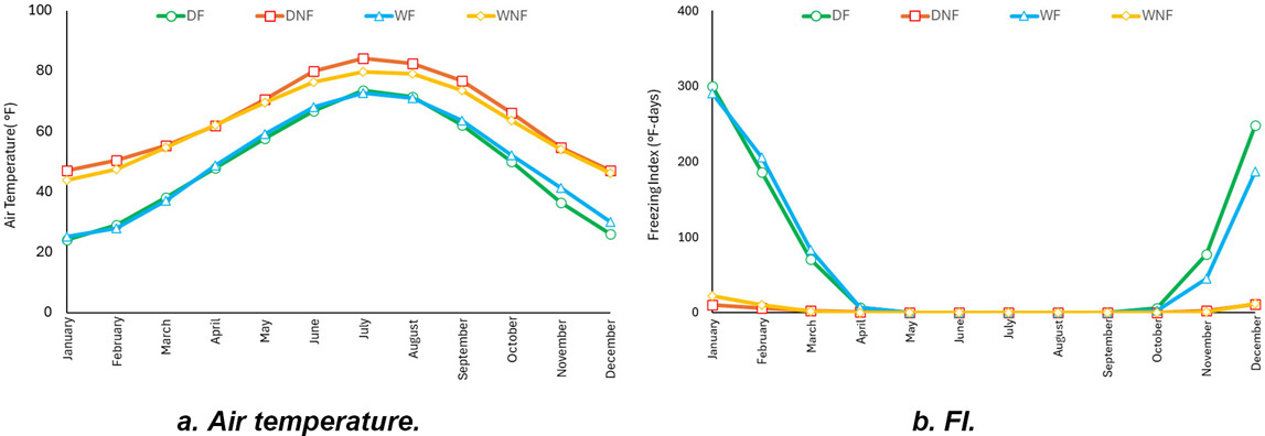
Precipitation did not follow the same behavior across all climatic zones. For DF and DNF climatic zones, a significant increase was observed from June to August, while WF and WNF climatic zones had more uniform precipitation distribution throughout the year (Figure 21).
Consecutive months were grouped into seasons for each climatic zone and SMP section based on having values below established limits for air temperature and FI. The grouping effort initially assumed four seasons (spring, summer, fall, and winter), and each season consisted of no more than 5 months. However, the climate data did not clearly differ between spring and fall seasons, therefore, consecutive months for winter and summer seasons were defined using the climatic data with fall and spring occurring between these two defined seasons (e.g., winter defined as December to March, summer defined as June to August; therefore, spring defined as April to May and fall defined as September to November). The winter season for the DF climatic zone was defined using the percent difference between the average FI (from all months) and the FI per month (Table 14).
Table 14. Season Criteria – DF Climatic Zone
| Season | Begin | End |
|---|---|---|
| Winter | |(FIi – FIAVG)/FIAVG | ≥ 0.50 | |(FIi – FIAVG)/FIAVG | < 0.50 |
| Spring | End of Winter | Start of Summer |
| Summer | |(Ti – TJul)/TJul| ≤ 0.25 | |(Ti – TJul)/TJul| > 0.25 |
| Fall | End of Summer | Start of Winter |
Notes: Flavg = Average seasonal FI (°F-days).
TJul = Average air temperature for July (°F).
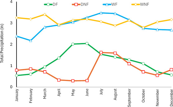
Using FI for a given month, for all sections, made it difficult to establish an absolute limit (e.g., 300, 400 or 500 °F-day) (Figure 22a). However, using the percent difference in FI from one month to the next, more significant changes in FI were noted (Figure 22b).

Figure 23 illustrates the mean air temperature by month for the SMP sections in the DF climatic zone. There’s no clear distinction of summer based on average monthly air temperature; therefore, the percent difference between the July temperature and the temperature for the other months was used to define the summer season (Figure 23b).
The winter and summer seasons for the WF climatic zone were defined using a similar approach as the DF climatic zone. However, the percent difference criteria were adjusted to reflect the northern climates (Table 15).
Table 15. Season Criteria – WF Climatic Zone
| Season | Begin | End |
|---|---|---|
| Winter | |(FIi – FIAVG)/FIAVG| ≥ 0.60 | |(FIi – FIAVG)/FIAVG| < 0.60 |
| Spring | End of Winter | Start of Summer |
| Summer | |(Ti – TJul)/TJul| ≤ 0.20 | |(Ti – TJul)/TJul| > 0.25 |
| Fall | End of Summer | Start of Winter |
The winter season for the DNF and WNF climatic zones could not be differentiated using the FI due to the relatively low monthly variation; therefore, the percent difference criteria was based on the comparison of the January air temperatures to all other months (Table 16 and Table 17 for DNF and WNF, respectively). For summer, the limit was reduced to a stricter value due to the closeness in air temperature between July and the rest of the months.
Table 16. Season Criteria – DNF Climatic Zone
| Season | Begin | End |
|---|---|---|
| Winter | |(Ti – TJan)/TJan| ≤ 0.25 | |(Ti – TJan)/TJan| > 0.25 |
| Spring | End of Winter | Start of Summer |
| Summer | |(Ti – TJul)/TJul| ≤ 0.05 | |(Ti – TJul)/TJul| > 0.05 |
| Fall | End of Summer | Start of Winter |
Notes: TJan = Average air temperature for January (°F).
Table 17. Season Criteria – WNF Climatic Zone
| Season | Begin | End |
|---|---|---|
| Winter | |(Ti – T1)/T1| ≤ 0.25 | |(Ti – T1)/T1| > 0.25 |
| Spring | End of Winter | Start of Summer |
| Summer | |(Ti – T7)/T7| ≤ 0.05 | |(Ti – T7)/T7| > 0.05 |
| Fall | End of Summer | Start of Winter |
Appendix E includes a summary of season definitions (by month) by SMP section.
AASHTO 1993 Guide Seasonal Adjustment Model
As described previously, the AASHTO 1993 Guide recommends two approaches for conducting seasonal adjustments: a laboratory relationship between moisture content and modulus and a seasonal deflection measurement method. Using the seasonal deflection measurement method, the subgrade resilient modulus
was determined for each LTPP SMP section. Prior to backcalculating the resilient moduli, data were filtered according to:
- Surface layer: The seasonal adjustment model was developed for asphalt pavements; therefore, concrete pavements were excluded from the analysis.
- Lane number: The FWD measurements for the outer wheel path was extracted for this analysis (refer to Figure 19). Data tested on the mid-lane was not included in the analysis. Typically, agencies conduct FWD testing in the outer wheel path due to traffic control restrictions (i.e., placing FWD equipment at mid-lane requires traffic control on adjacent lanes).
- Drop height: Deflections associated with 6,000, 9,000, 12,000, and 15,000 lbs (drop heights one through four, respectively) were extracted. An analysis of variance (ANOVA) was conducted to determine if the applied load had a significant influence on the backcalculated moduli. The variance across the means between drop heights two through four was determined. Not all FWD tests included drop height one. A p-value of 0.05 was used to assign statistical significance. The analysis indicated the layer moduli did not significantly differ by drop height (Table 18 and Figure 24). Therefore, a drop height equivalent to 9,000 lbs. was used in the analysis.
Table 18. ANOVA Results – p-values
| Scenario | Asphalt | Gravel Base | Subgrade |
|---|---|---|---|
| Drop height 1 to 4 | 0.06 | 0.00 | 0.03 |
| Drop height 2 to 4 | 0.59 | 0.08 | 0.39 |

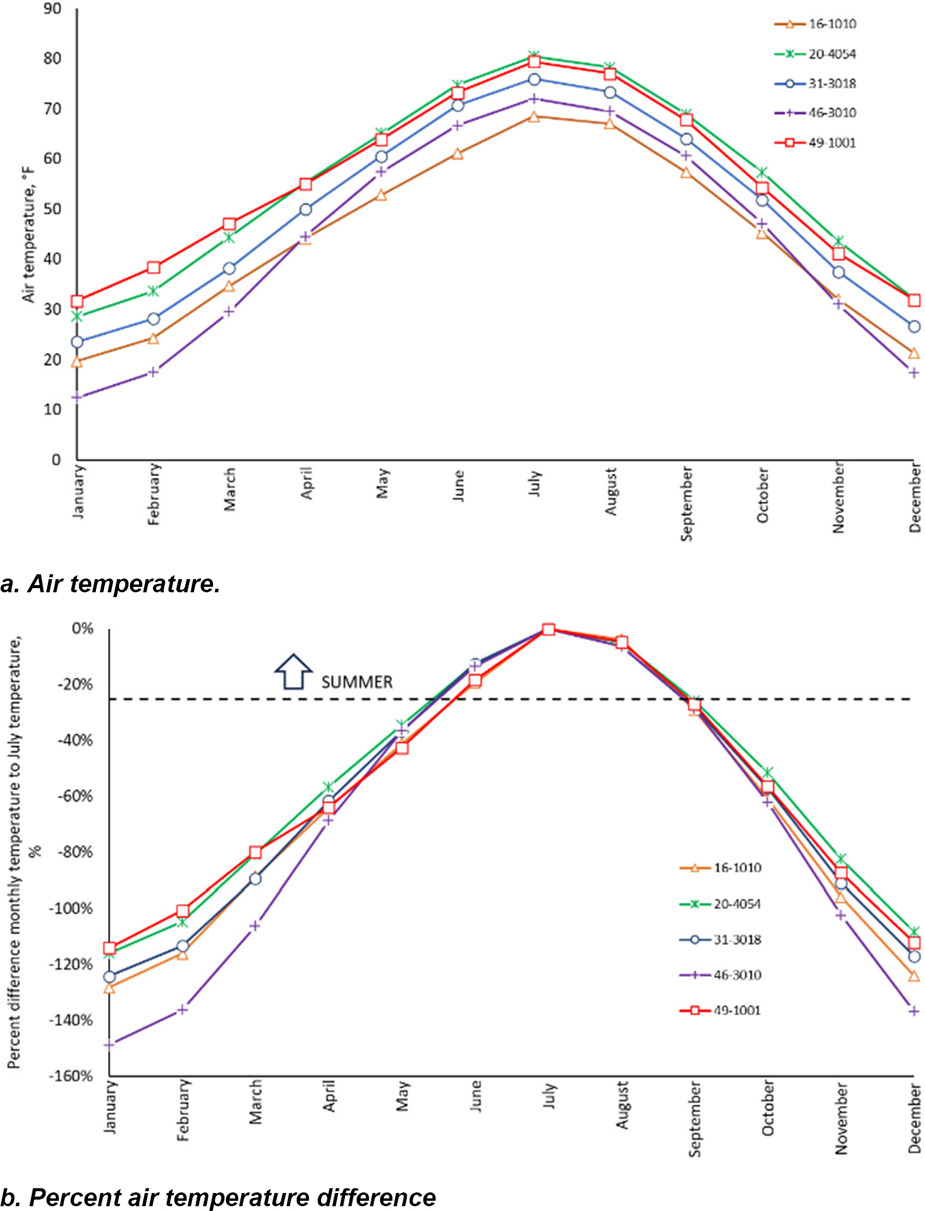
- Non-decreasing deflection: FWD tests with deflection values at a sensor offset “Si” greater than deflection values at a sensor closer to the point of force application “Si-1” were removed from the analysis. Figure 25 illustrates an example of two deflection basins measured at the same location, approximately 1 month apart. The FWD test performed in December 1993 shows a discontinuity (i.e., lower deflection) at 18 inches compared to the deflections measured at 8 and 24 inches. In comparison, the deflections measured in January 1994 show a more typical progressive decline in deflection with an increase in sensor offset distance.
Table 19 provides a summary of deflection basins, by climatic zone, used in the analysis.
Table 19. Summary of Deflection Basins by Climatic Zone
| Climatic Zone | Total No. of Deflection Basins1 | No. of Deflection Basins Removed2 | No. of Deflection Basins Used |
|---|---|---|---|
| DF | 1,111,935 | 985,820 | 126,115 |
| DNF | 577,155 | 505,487 | 71,668 |
| WF | 2,754,773 | 2,443,380 | 311,393 |
| WNF | 1,219,913 | 1,078,147 | 141,766 |
| Total | 5,663,776 | 5,012,834 | 650,942 |
1 Includes all FWD tests.
2 Tests removed included middle-lane (F1), drop heights 1, 3, and 4, and non-decreasing deflection pattern.
The subgrade resilient modulus from a single deflection measurement is expressed as (AASHTO 1993):
| (Eq. 38) |
where:
| MR = | subgrade resilient modulus (psi) |
| P = | applied load (lb) |
| dr = | deflection at a distance r from the center of the load (in.) |
| r = | distance from center of load (in.) |
The LTPP database expressed the applied load in terms of pressure. To migrate from pressure to load, the following equation was used.
| (Eq. 39) |
where:
| P = | applied load (lb) |
| σ = | applied stress (psi) |
| A = | FWD load plate area (in2), a plate radius of 6 in. was used at all LTPP FWD testing locations) |
The subgrade resilient modulus calculation was repeated at every sensor offset by modifying the distance from the center of load (e.g., 24 in., 36 in., 48 in.) and the lowest resulting value was selected to represent the subgrade resilient modulus for each testing point. A subgrade modulus adjustment factor, normalized to the summer resilient modulus, was determined for the spring, fall and winter modulus using the following equation:
| (Eq. 40) |
where:
| Fseason = | adjustment factor for spring, fall or winter |
| MR Season = | resilient modulus for spring, fall or winter (psi) |
| MR Summer = | resilient modulus for summer (psi) |
The modulus adjustment factor was determined for each state by averaging the corresponding seasonal factor for each SMP section within that state. As an example, Table 20 includes the calculated subgrade resilient modulus, and section and state adjustment factors for the three asphalt-surfaced SMP sections in Minnesota. For these sections, the maximum subgrade resilient modulus occurs during the winter months (e.g., frozen condition) and the lowest subgrade resilient modulus occurs during the fall months.
Table 20. Example of Subgrade Resilient Modulus (Minnesota)
| Section | Average Subgrade Modulus (psi)1 | Seasonal Adjustment Factor | ||||||
|---|---|---|---|---|---|---|---|---|
| Spring | Summer | Fall | Winter | Spring | Summer | Fall | Winter | |
| 27-1018 | 26,183 (14,626) | 20,063 (509) | 18,427 (912) | 75,938 (44,311) | 1.31 | 1.00 | 0.92 | 3.79 |
| 27-1028 | 30,179 (14,882) | 22,577 (363) | 20,759 (258) | 58,832 (23,120) | 1.34 | 1.00 | 0.92 | 2.61 |
| 27-6251 | 37,765 (13,543) | 30,576 (538) | 27,915 (979) | 74,900 (46,517) | 1.24 | 1.00 | 0.91 | 2.45 |
| Statewide | 31,376 (5,883) | 24,405 (5,490) | 22,367 (4,944) | 69,890 (9,591) | 1.29 | 1.00 | 0.92 | 2.95 |
1 Standard deviation is shown in parenthesis.
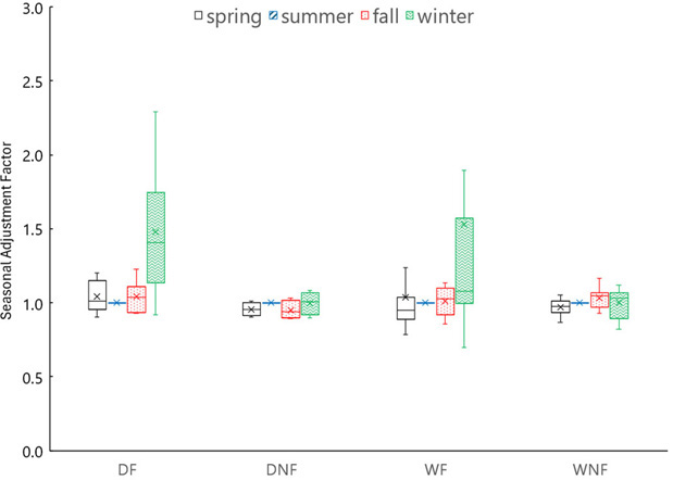
The ranges in seasonal subgrade adjustment factors for each climatic zone are presented in Figure 26 (Appendix F provides the subgrade seasonal adjustment factors for each SMP section). As expected, the
WF and DF climatic zones tend to have greater variability in the seasonal adjustment factor compared to the WNF and DNF climatic zones.
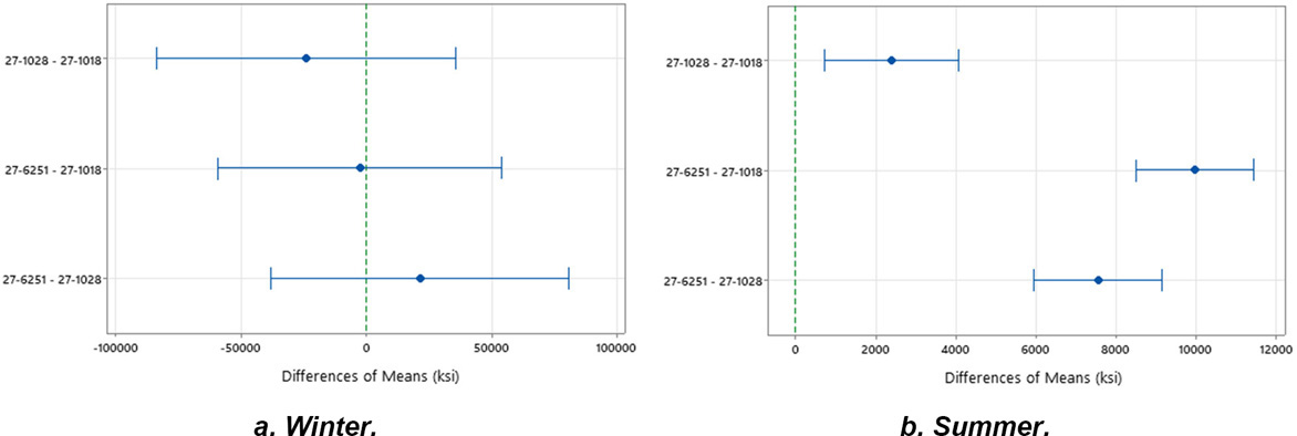
States containing two or more SMP sections were further analyzed using ANOVA with post-hoc Tukey comparison to determine whether a state’s adjustment factor could be accurately applied regardless of FWD testing location within the state. Of the 10 states with two or more asphalt-surfaced SMP sections, only Alabama, Arizona, Minnesota, New Jersey, and Texas had sections where the difference in means was not statistically significant. As an example, Figure 27 illustrates the Tukey method results for the Minnesota SMP sections for the difference of subgrade resilient modulus means for winter and summer seasons. The average difference in means between the two sections listed for each row on the y-axis is represented by the blue dots, while the whiskers depict the confidence interval (95%). If the 95% confidence interval does not include zero, it implies the difference in moduli between the two sections is significantly different and a single statewide adjustment factor would not be appropriate. If the whisker range includes zero, it means that the means are statistically the same (x?1 = x?2), and a statewide adjustment factor would be appropriate.
Enhanced Integrated Climatic Model
To quantify the climatic conditions at the SMP sections using the EICM, the required PMED inputs were extracted from the LTPP database tables. If data were missing, the PMED default parameters were used. Table 21 summarizes the required PMED inputs and the LTPP table references. The inputs for layer type, layer thickness, subgrade soil classification, and construction data for each SMP section are included in Appendix G.
This analysis intended to only extract the outputs from the EICM and not those for pavement design purposes.
Table 21. PMED Input Parameters
| Input Category | Consideration |
|---|---|
| Traffic |
Default:
|
| Climate | Closest climate station to the SMP section (MERRA data) |
| Pavement Structure | Type: new Pavement type: flexible pavement Design life: 20 years Traffic operation date: first FWD test Asphalt binder grade: PG 64-22 |
The PMED generates intermediate files containing relevant information regarding the modulus adjustment factors and moisture contents on a month/sub-month basis for each granular and subgrade sublayer. PMED also generates intermediate files with modulus variation for all sublayers over the design period (Table 22).
Table 22. PMED intermediate Files
| File name | Intermediate file content | Frequency |
|---|---|---|
| space.dat |
| Monthly |
| modulus.tmp (asphalt designs only) |
| Sub-monthly |
| PCCModulus.txt (concrete only) |
| Monthly |
| thermal.tmp |
| Hourly |
The PMED modulus adjustment factors were averaged by season using the information contained in the space.dat intermediate file. The modulus adjustment factors for the aggregate base and the subgrade layer were averaged for all sublayers within the corresponding layer. Since PMED adjustment factors are not normalized to the seasons or months (e.g., summer values could be different from 1.0), the output factors were changed to reflect a similar pattern as the AASHTO 1993 Guide criteria. Of the 85 SMP sections, 63 sections included an aggregate base, and the remaining 22 sections included an asphalt- or cementitious-treated base (modulus adjustment factor was set to 1.0) or no base at all.
For the asphalt layer, the modulus.tmp intermediate file was used. The adjustment factor was calculated by normalizing the seasonal modulus to the summer modulus value. Figure 28 illustrates the asphalt layer seasonal adjustment factors for all climatic zones. The average asphalt layer adjustment factor was similar for each season regardless of the climatic zone. However, asphalt layer modulus adjustment factors for SMP sections in the WF and WNF climatic zones had a wider range for the winter seasons than those in the DF and DNF climatic zones.

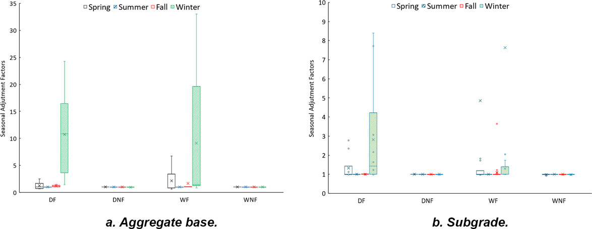
As expected, the DF and WF climatic zones had significantly higher modulus adjustment factors for the winter season compared to the DNF and WNF climatic zones (Figure 29a). The average aggregate base modulus adjustment factor for the DF and WF climatic zones was approximately 10. However, the interquartile range for the DF climatic zone ranged from 3 to 16 with a maximum value of 23, while the WF climatic zone modulus adjustment factor ranged from 1 to 20 with a maximum value of 35. The median value of the DF climatic zone was equal to the mean of the WF climatic zone. In the WF climatic zone, 50% of the WF adjustment factors for winter were below 1.5 while 50% of the DF adjustment factors for winter were below 10. The high range in the WF climatic zone was caused by the higher adjustment factors for the SMP sections in Minnesota and Canada.
The results for the subgrade layer are similar to those for the aggregate base; however, the average modulus adjustment factor for the DF and WF climatic zones was 3 and 8, respectively (Figure 29b). The DF climatic zone has more sections with a significantly high adjustment factor. In addition, the upper quartile adjustment factor for the WF climatic zone (i.e., 75% of the data) was below 1.4 while the DF climatic zone reached adjustment factors of 4.2.
For the concrete surface layer, the seasons did not significantly affect adjustment factors in any of the climatic zones (i.e., all adjustment factors were 1.0). This is expected as PMED predicts a continuous elastic modulus increase during the first curing days, followed by an asymptotic behavior once the design strength has been reached.
Appendix H includes the seasonal layer modulus adjustment factors for each asphalt pavement SMP section.
Comparison of AASHTO 1993, EICM, and LTPP
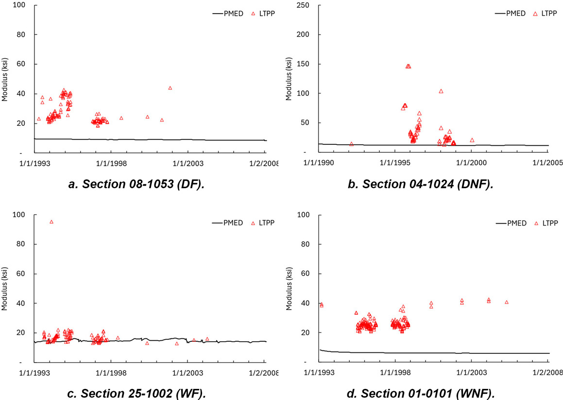
Due to significant variation in adjustment factors for the SMP sections in climates with freezing conditions, a comparison was made between the PMED predicted and LTPP backcalculated layer moduli. Four sections, with considerable numbers of data points over the study period, were selected from each climatic zone to illustrate the results of the comparison (all results are provided in Appendix I). It is important to emphasize that while the FWD tests were performed at multiple hours, locations, and times of the year, PMED predicts a single monthly value at a constant interval; therefore, prohibiting a point-to-point comparison.
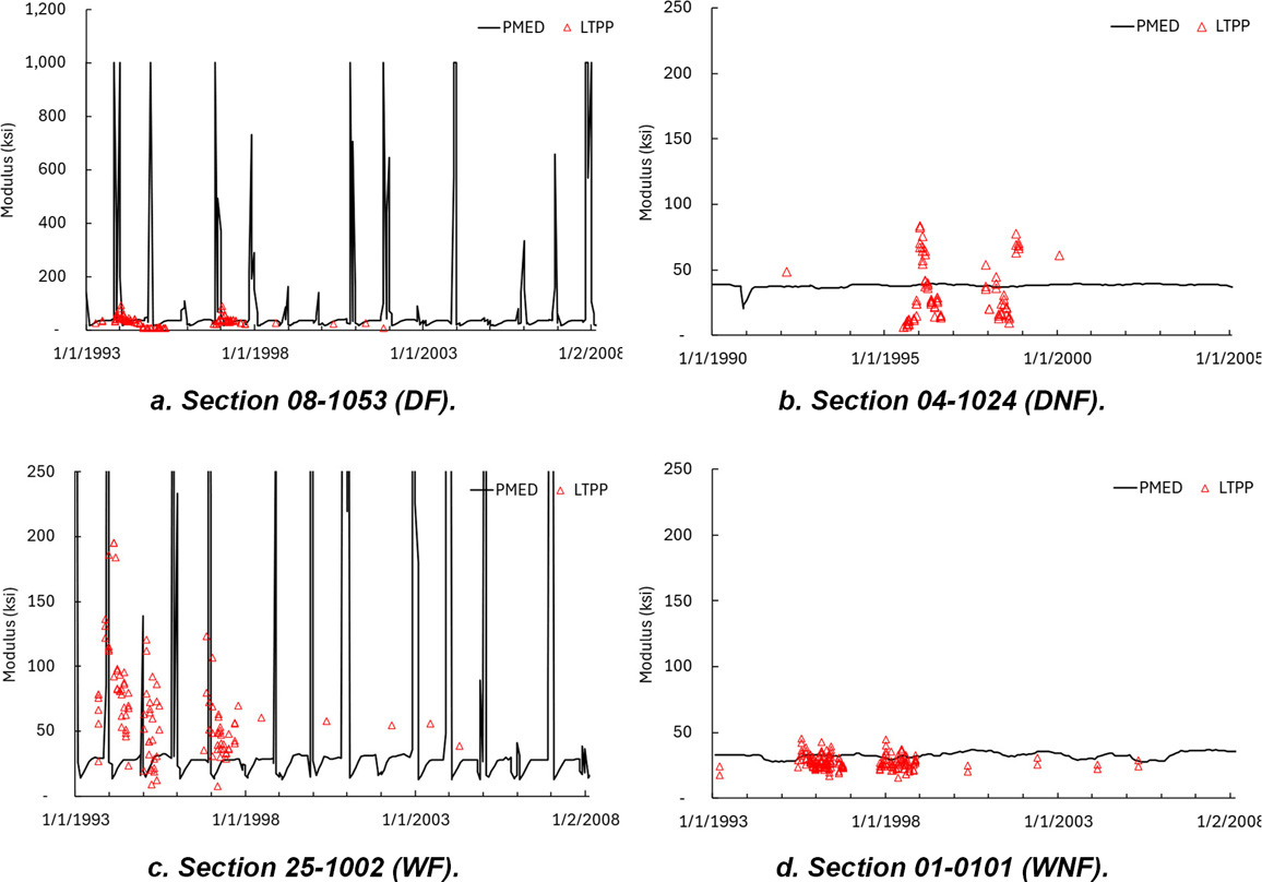
Figure 30 illustrates a comparison of the PMED predicted and the LTPP backcalculated aggregate base moduli for the DF, DNF, WF, and WNF climatic zones. The peaks seen in Sections 08-1053 and 25-1002 depict the maximum modulus PMED applied during winter due to the temperature and moisture content. For DF and WF climatic zones, the PMED-predicted module was significantly more variable (and higher) compared to the LTPP backcalculated moduli. A significant difference in aggregate base layer modulus appears for the DF and WF climatic zones. In these cases, PMED predicted a maximum aggregated base modulus of 1,000,000 psi during the coldest months. For Section 08-1053, the PMED-predicted aggregate base modulus was nearly 50 times higher during August-September than the LTPP backcalculated aggregate base layer moduli. For Section 25-1002, the PMED-predicted aggregate base layer moduli were nearly 10 times the LTPP backcalculated aggregate base layer moduli in November and December.
Similarly, Figure 31 compares the PMED predicted and LTPP backcalculated subgrade moduli for the same SMP sections. The PMED-predicted subgrade moduli were closer to the LTPP backcalculated moduli compared to those of the aggregate base layer. In all cases, the LTPP backcalculated subgrade modulus was higher than the PMED predicted modulus, averaging 35,000 to 40,000 psi and 15,000 to 20,000 psi, respectively.
The average moduli and standard deviations determined from the AASHTO 1993, PMED, and LTPP methods, by climatic zone, are summarized in Table 23 to Table 25 for the asphalt layer, base layer, and subgrade, respectively.
Table 23. PMED and LTPP Average Moduli and Standard Deviations – Asphalt Layer
| Average Modulus (ksi) | Standard Deviation (ksi) | ||||||||
|---|---|---|---|---|---|---|---|---|---|
| Climatic Zone | Method | Spring | Summer | Fall | Winter | Spring | Summer | Fall | Winter |
| DF | PMED | 1,695 | 1,180 | 2,897 | 3,095 | 847 | 415 | 338 | 95 |
| LTPP | 1,047 | 456 | 1,277 | 3,488 | 847 | 259 | 957 | 2,790 | |
| WF | PMED | 1,682 | 900 | 2,554 | 3,071 | 720 | 306 | 630 | 147 |
| LTPP | 1,006 | 514 | 1,097 | 3,267 | 856 | 268 | 1,094 | 2,870 | |
| DNF | PMED | 1,336 | 892 | 2,449 | 2,759 | 612 | 315 | 574 | 329 |
| LTPP | 975 | 583 | 932 | 1,411 | 495 | 243 | 556 | 634 | |
| WNF | PMED | 992 | 716 | 1,993 | 2,413 | 574 | 244 | 683 | 568 |
| LTPP | 835 | 1,268 | 1,255 | 2,325 | 857 | 1,935 | 1,511 | 1,828 | |
Table 24. PMED and LTPP Average Moduli and Standard Deviations – Base Layer
| Average Modulus (ksi) | Standard Deviation (ksi) | ||||||||
|---|---|---|---|---|---|---|---|---|---|
| Climatic Zone | Method | Spring | Summer | Fall | Winter | Spring | Summer | Fall | Winter |
| DF | PMED | 29 | 36 | 111 | 285 | 8 | 2 | 198 | 339 |
| LTPP | 21 | 17 | 24 | 86 | 20 | 8 | 30 | 81 | |
| WF | PMED | 40 | 30 | 91 | 280 | 102 | 3 | 214 | 384 |
| LTPP | 27 | 26 | 27 | 74 | 26 | 13 | 30 | 78 | |
| DNF | PMED | 39 | 39 | 39 | 39 | 1 | 1 | 1 | 2 |
| LTPP | 24 | 34 | 23 | 26 | 15 | 25 | 16 | 16 | |
| WNF | PMED | 33 | 34 | 33 | 34 | 3 | 3 | 3 | 3 |
| LTPP | 26 | 47 | 31 | 32 | 22 | 49 | 30 | 29 | |
Table 25. PMED, LTPP, and AASHTO 1993 Average Moduli and Standard Deviations – Subgrade
| Average Modulus | Standard Deviation | ||||||||
|---|---|---|---|---|---|---|---|---|---|
| Climatic Zone | Method | Spring | Summer | Fall | Winter | Spring | Summer | Fall | Winter |
| DF | PMED | 30 | 11 | 12 | 45 | 5 | 5 | 10 | 71 |
| LTPP | 30 | 27 | 30 | 59 | 22 | 18 | 22 | 44 | |
| AASHTO | 17 | 16 | 17 | 23 | 7 | 6 | 6 | 9 | |
| WF | PMED | 36 | 13 | 26 | 134 | 129 | 4 | 89 | 281 |
| LTPP | 50 | 48 | 42 | 64 | 73 | 80 | 53 | 69 | |
| AASHTO | 27 | 24 | 26 | 37 | 15 | 7 | 8 | 26 | |
| DNF | PMED | 17 | 19 | 17 | 18 | 6 | 6 | 6 | 6 |
| LTPP | 36 | 47 | 47 | 47 | 15 | 17 | 35 | 29 | |
| AASHTO | 28 | 34 | 27 | 10 | 9 | 11 | 10 | 9 | |
| WNF | PMED | 13 | 13 | 13 | 14 | 6 | 6 | 6 | 6 |
| LTPP | 33 | 29 | 38 | 25 | 23 | 23 | 29 | 14 | |
| AASHTO | 22 | 23 | 23 | 22 | 10 | 13 | 10 | 13 | |
An ANOVA was used to compare the average layer moduli from AASHTO 1993, PMED, and LTPP for each layer, climatic zone, and season. For AASHTO 1993, only the subgrade moduli were applicable to this analysis. As shown in Table 26 and Table 27, in most cases, the means were significantly different between AASHTO 1993 and LTPP and between PMED and LTPP.
Table 26. ANOVA Layer Modulus Results AASHTO 1993 vs LTPP
| Climatic Zone | Spring | Summer | Fall | Winter |
|---|---|---|---|---|
| DF | SD | SD | SD | SD |
| WF | SD | SD | SD | SD |
| DNF | SD | SD | SD | SD |
| WNF | SD | NSD | SD | NSD |
Note: SD – statistically different and NSD – not statistically different.
Table 27. ANOVA Results PMED vs LTPP Layer Moduli
| Climatic Zone | Layer | Spring | Summer | Fall | Winter |
|---|---|---|---|---|---|
| DF | Asphalt | SD | SD | SD | SD |
| Base | SD | SD | SD | SD | |
| Subgrade | SD | SD | SD | NSD | |
| WF | Asphalt | SD | SD | SD | SD |
| Base | NSD | SD | SD | SD | |
| Subgrade | NSD | SD | SD | SD | |
| DNF | Asphalt | SD | SD | SD | SD |
| Base | SD | SD | SD | SD | |
| Subgrade | SD | SD | SD | SD | |
| WNF | Asphalt | SD | SD | SD | NSD |
| Base | SD | SD | SD | NSD | |
| Subgrade | SD | SD | SD | SD |
Note: SD – statistically different and NSD – not statistically different.
Potential differences between AASHTO 1993, LTPP, and PMED layer moduli values may be a function of several factors. The AASHTO 1993 procedure was based on the conditions from the AASHO Road Test in Ottawa, IL. The results of the Road Test were compiled and assessed for application to other roadway locations and conditions. The AASHTO 1993 method also adjusts subgrade moduli using a relative damage factor which may vary depending on-site-specific conditions from those estimated from the AASHO Road Test. The backcalculated layer moduli contained within the LTPP database were generally determined using a pavement model consisting of a surface layer (asphalt or concrete), a base layer (e.g., gravel base, cementitious base, asphalt base), and two subgrade layers. However, other pavement models (e.g., use of stiff layer, two-layer system) may have resulted in improved layer moduli estimates. For the PMED analysis conducted in this study, different pavement models were evaluated to generate more reasonable layer moduli values. Finally, the PMED analysis provides layer moduli for each day and month of the performance period. In contrast, some of the LTPP sections did not have layer moduli for all months of the evaluation period.


