LTPP Data Analysis: Improving Use of FWD and Longitudinal Profile Measurements (2024)
Chapter: 6 Longitudinal Profile Analysis and Adjustment
CHAPTER 6
Longitudinal Profile Analysis and Adjustment
Asphalt Pavements
The longitudinal profile data for the asphalt pavement SMP sections was analyzed to assess the applicability of seasonal adjustments. The time-series IRI data was plotted, and a linear regression was fitted to the data (Figure 42).
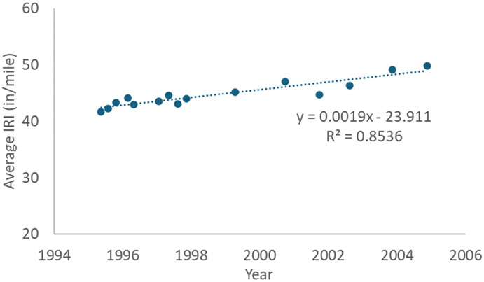
The analysis period varied for each asphalt pavement SMP section but generally began with the first measurement after construction. The analysis period ended when maintenance or rehabilitation work was performed and impacted the IRI (i.e., patching, asphalt overlay). The seasons defined in Chapter 4 were applied to this analysis. A difference factor between the measured and regression-calculated IRI was determined and divided by the measured IRI value for each measurement (i.e., normalized).
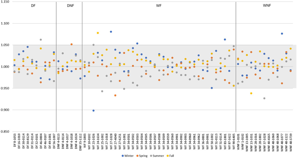
Figure 43 illustrates the difference factor for each profile measurement for each SMP section. An adjustment factor greater than 1.0 indicates the measured IRI value was less than the regression IRI value. The available SMP asphalt pavement longitudinal profile data did not show significant seasonal effects, most of the observed seasonal variations were less than 5%. There also appears to be no systematic difference between WF and any other climatic zones, except for the few sections that are most likely thin or weak designs on expansive clay (e.g., 23-1026, 33-1001).
While seasonal effects may exist, large effects were not observed to justify an algorithmic seasonal adjustment and, over a limited set of conditions, showed the seasonal effects are small for asphalt pavement SMP sections.
Concrete Pavements
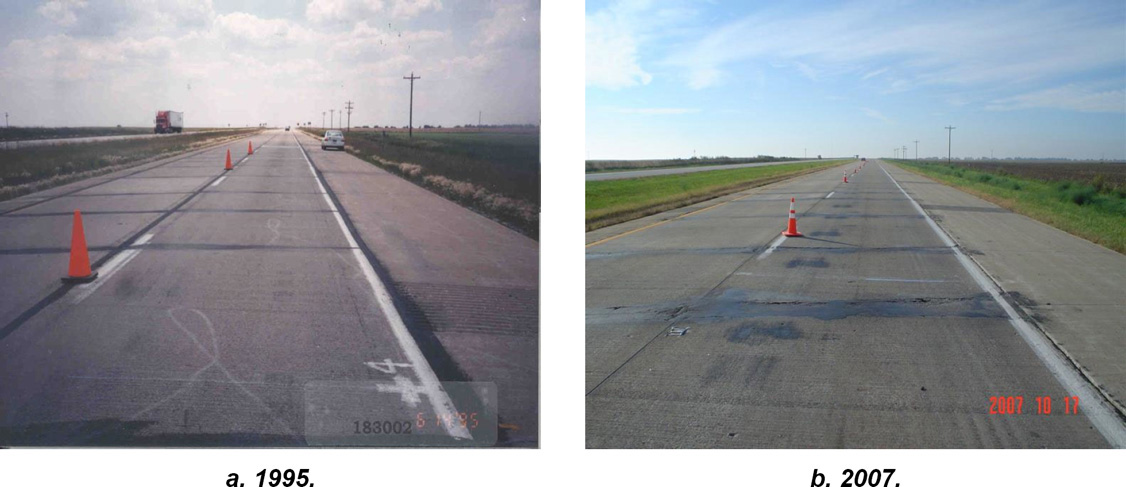
For concrete pavements, slab curvature, joint movement, and other types of deterioration can significantly impact IRI. For example, IRI measurements for Section 18-3002 demonstrate a rapid change in IRI over a relatively brief period (Figure 44). IRI measurements for Section 18-3002 remained constant from 1990 to 2000 (average IRI 115 in/mi). However, the IRI quickly increased to approximately 190 in/mi by 2011. Based on the LTPP reports and photo logs, joint deterioration progressed over the evaluation period, altering the pavement’s original profile (Figure 45). Two major maintenance events occurred and included partial depth patching (2009) at joints and concrete fracture treatment to reduce pavement roughness.

Characterizing temporal and diurnal temperature and moisture impacts on JPCP requires more analysis. The following further discusses and applies the 2GCI method for analyzing JPCP curling and warping.
2GCI Method
As noted in Chapter 2, the 2GCI method estimates the IRI that would exist in the absence of slab curl and warp. It does so by using an empirical estimate of the relationship between deformation caused by curl and warp and IRI. Slab deformation is quantified using a slab-by-slab analysis of longitudinal profiles, in which the profile of each slab is fitted to an assumed slab profile caused by curl and warp. In most implementations, the assumed slab profile corresponds to the Westergaard model (Westergaard 1926, 1927). The Westergaard model predicts vertical deformation along a slab, given a constant vertical strain gradient and structural properties (slab length, radius of relative stiffness, and Poisson’s ratio). In the 2CGI analysis, the structural properties and the measured slab profile are provided as inputs, and a curve fitting procedure returns the PSG. The PSG value assigned to a test section is the average PSG for the slabs within that section.
Estimating the relationship between PSG and IRI requires analysis of profiles measured over temporal and diurnal cycles, in which significant changes in roughness associated with changes in curl and warp are present. The IRI-PSG relationship is applied over the long term to remove the influence of curl and warp on IRI using the PSG from each profile.
Case Example: Ohio SMP 39-0204
The following example illustrates the 2GCI method for SMP Section 39-0204. SMP Section 39-0204 is in Ohio, on US 23 (northbound), approximately 35 miles north of Columbus, Ohio. The highway is classified as a rural principal arterial and is in the WF climatic zone. The pavement structure consisted of 11.1 in. JPCP, 5.8 in. crushed stone, and silty clay subgrade (Figure 46). Over the performance period, a total of 24 slabs had transverse cracking, one slab had a corner break, minimal faulting, and no joint spalling.

Longitudinal profile data were collected from 1996 to 2006, totaling 17 visits (Table 43). Noted observations included seasonal changes in profile over 2 years early in the life of the section, as well as changes throughout the day on the seasonal visits (e.g., March 1998, November 1998, June 2000). Five repeated passes were conducted for each visit. The profiles were selected from raw data and longitudinally aligned as described by Karamihas et al. (2023).
Table 43. Profile Measurement Visits (Section 39-0204).
| Age (years) | Date | Time |
|---|---|---|
| 0.24 | 12/27/1996 | 10:22 |
| 1.19 | 12/08/1997 | 09:34 |
| 1.43 | 03/07/1998 | 06:12, 11:20, 15:06 |
| 1.65 | 05/28/1998 | 06:23, 15:06 |
| 1.86 | 08/13/1998 | 03:22, 07:31 |
| 2.11 | 11/12/1998 | 09:24, 15:01 |
| 2.44 | 03/10/1999 | 06:25, 14:00 |
| 2.72 | 06/22/1999 | 06:14, 15:32 |
| 3.05 | 10/20/1999 | 08:54 |
| 3.71 | 06/17/2000 | 05:23, 14:35 |
| 3.88 | 08/16/2000 | 09:17 |
| 5.09 | 11/04/2001 | 08:30 |
| 6.18 | 12/06/2002 | 11:36 |
| 6.58 | 4/29/2003 | 14:19 |
| 7.34 | 02/04/2004 | 15:12 |
| 8.59 | 05/05/2005 | 12:37 |
| 9.85 | 08/08/2006 | 12:10 |
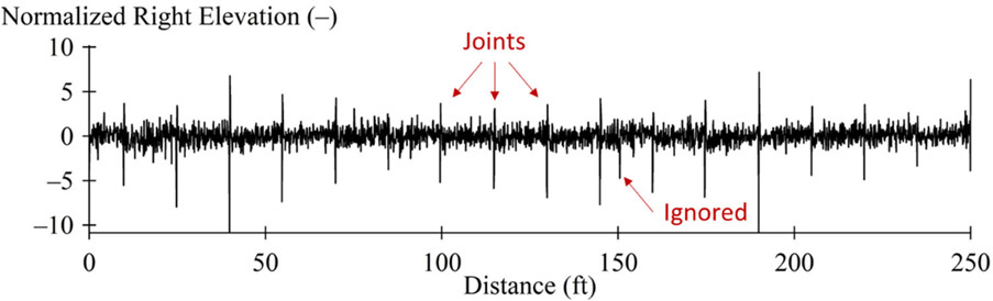
Step 1: Find the transverse joint locations.
The joint finding procedure identifies the downward spikes in the profile measurements corresponding to the transverse joints. A high-pass filter with a short cut-off was used to help identify the spikes. Figure 47 shows an example of the first 250 feet of profile for the right wheel path collected on October 20, 1999. The high-pass filtered profile was normalized by its root mean square value and a threshold was used to identify candidate joint locations at the downward spikes. In some cases, downward spikes that do not fit the expected joint spacing are ignored, such as the spike at 150 feet.
The application of a spike detection algorithm to production profile measurements for pavement network monitoring may not always succeed, depending on the sampling rate, filtering procedures, and profile height sensor footprint. Spike detection may also fail on pavements with narrow gaps at the joints. However, other options are available based on examination of localized change in slope and curvature (see Byrum 2009, Nazef et al. 2009, 2010, Chang et al. 2012, and Agurla and Lin 2015).
Step 2: Fit each slab profile to an assumed slab shape.
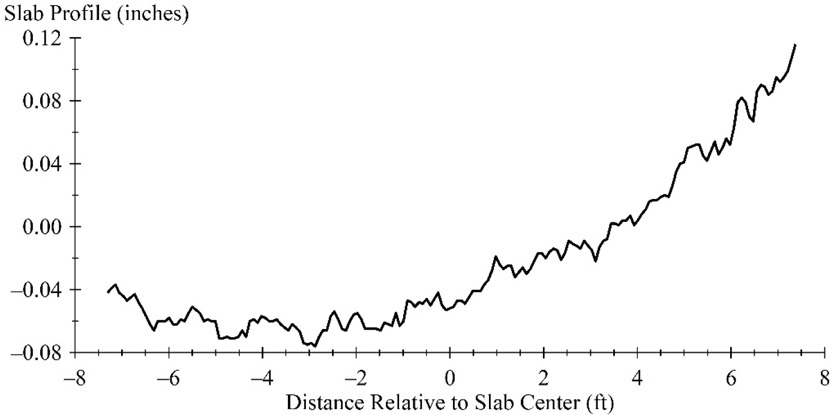
Isolate each slab profile using the joint locations from the previous step. Figure 48 shows the right wheel path profile of the 17th slab (the last slab identified in Figure 47) extracted from a pass collected on October 20, 1999. The longitudinal distance was reset with an origin at the center of the slab.
To avoid including downward spikes at the joints, about 2 inches of profile was eliminated at the slab boundaries. Before applying the curve fitting procedure, the profile was detrended and then offset vertically so that the mean elevation was zero. Figure 49 shows the profile after it was detrended and offset vertically.
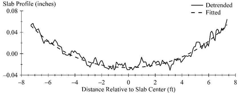
The dashed or “Fitted” line in Figure 49 represents the Westergaard fitted curve and is determined using:
| (Eq. 54) |
where,
| PSG = | pseudo-strain gradient (microstrain per in.) |
| λ = | |
| l = | radius of relative stiffness (in.) |
| b = | slab length (in.) |
| µ = | Poison’s ratio (unitless) |
| x = | longitudinal distance from the slab center (in.) |
| z = | fitted profile (in.) |
The procedure requires an estimate of Poisson’s ratio and radius of relative stiffness. In this example, Poisson’s ratio was assumed to be 0.15. The radius of relative stiffness was obtained using information from the LTPP database, including slab thickness, and using the FWD data and the best-fit method to estimate the concrete elastic modulus and the modulus of subgrade reaction (Khazanovich et al. 2000):
| (Eq. 55) |
where,
| l = | radius of relative stiffness (in.) |
| E = | concrete elastic modulus (psi) |
| h = | slab thickness (in.) |
| µ = | Poison’s ratio (unitless) = 0.15 |
| k = | modulus of subgrade reaction (lb/in3) |
In this example, the radius of relative stiffness was 41.3 in. and the resulting PSG value for the profile of the right wheel along this slab was -30.17 microstrain/in.
Step 3: Aggregate the PSG values for each profile measurement.
For each wheel path profile, assemble a weighted average of the PSG values of individual slabs. Weight each PSG value by the portion of the slab length that appears within the test section boundaries.
Figure 50 illustrates the PSG values for the right wheel path profile. Thirty-two of the PSG values were generated for slabs that were within the test section. Those PSG values get full weighting. Two of the PSG values were generated for slabs that straddled the test section limits. Those PSG values get partial weighting. The segment-wide, weighted PSG value for the right wheel path profile measured on this pass was -29.09 microstrain/in. If repeated passes from each visit are available, average the segment-wide PSG values from each profile. Most applications of the 2GCI method have been demonstrated using five or more passes for each visit.

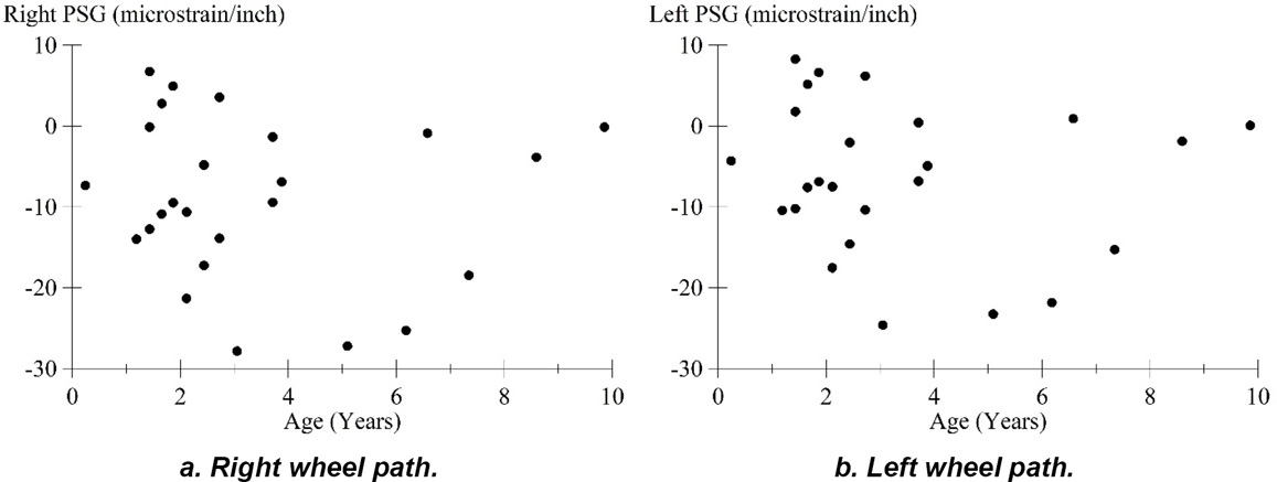
Figure 51 show the segment-wide PSG values for the left and right wheel paths versus pavement age for all 22 visits of Section 39-0204. Note that some pairs or triplets of values appear with the same age. Those were produced using two or more visits at different times within the same 24-hour period.
Step 4: Calculate the IRI values for each wheel track in each visit.
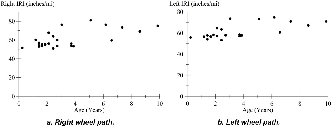
Figure 52 illustrates the right and left wheel path measured IRI versus pavement age for all 25 visits of Section 39-0204. IRI values were averaged for five passes from each visit.
Step 5: Establish the relationship between IRI and PSG.
Relate changes in IRI to changes in PSG using passes collected over a short time interval (e.g., 12-hour period) under varying environmental conditions. Significant changes in curl and warp are needed to get useful information in this step. Fit the following equation to observations on IRI versus PSG:
| (Eq. 56) |
where,
| IRI = | IRI value from each visit |
| PSG = | PSG value from each visit |
| dIRI/dPSG = | defines the effect of PSG on the IRI |
| IRIBack = | roughness not attributed to curl and warp for the visits included in the short-term analysis |
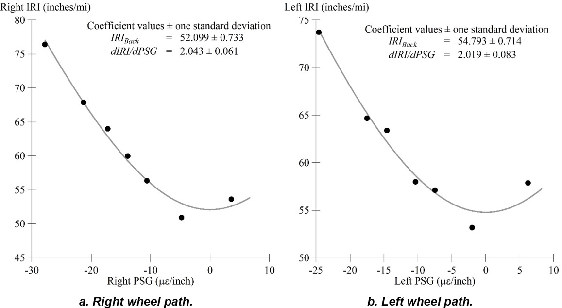
The dIRI/dPSG and IRIBack values are outputs of the fitting equation. The value of dIRI/dPSG is used to infer the value of IRIBack for other visits based on the PSG. Figure 53 illustrates the application of Equation 54 for the left and right wheel paths for seven visits to Section 39-0204 between November 12, 1998, and October 20, 1999. Each figure displays the fitted parameters.
Step 6: Apply the IRI-PSG relationship to other visits.
Once the estimate of dIRI/dPSG is obtained, it is used to remove the influence curl and warp from the IRI measured in other visits. That is, the following equation is applied to obtain IRIBack from each visit:
| (Eq. 57) |
where,
| IRIBack = | roughness not attributed to curl and warp |
| IRI = | obtained from Step 4 |
| PSG = | obtained from Step 3 |
| dIRI/dPSG = | obtained from Step 5 |
Figure 54 illustrates the right IRIBack and left IRIBack wheel path values versus pavement age for all 25 visits. This represents the long-term trend in roughness not associated with curl and warp. The trends are much more orderly than the trends in overall IRI shown in Figure 52. Examination of Figure 54 may reveal changes in roughness caused by distress more readily than examining overall IRI.
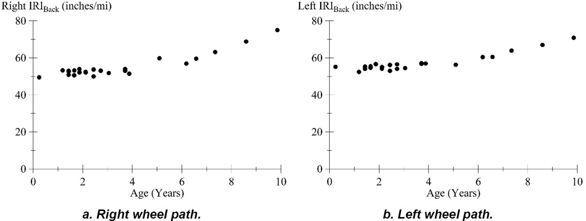
The approach demonstrated in this example provides an estimate of the development of roughness over time without the influence of curl and warp. However, not all the roughness removed is due to temporal or diurnal changes. Often, roughness caused by curl and warp develops gradually over several years.


