LTPP Data Analysis: Improving Use of FWD and Longitudinal Profile Measurements (2024)
Chapter: 5 FWD Deflection Analysis and Adjustment
CHAPTER 5
FWD Deflection Analysis and Adjustment
An FWD measurement descriptive analysis was conducted for each test, each visit with repeated daily tests, and tests at different days/seasons. The descriptive analyses included an assessment of deflection basin factors, backcalculated layer moduli, and repeatability, identification of outliers, and comparison of daily measurements. In addition, the descriptive analysis was used to determine which deflection parameters are most influenced by climatic variation.
Deflection Basin Factors
The temperature- and stiffness-dependence of the various deflection basin shapes were identified, including:
- AREA value. A calculation of the normalized area of a deflection basin, which is proportional to the ratio of the pavement stiffness (a function of thickness and material strength) to the subgrade stiffness.
- F1 shape factor. A calculation of a normalized representation of the amount of curvature in the deflection basin, which is inversely proportional to the ratio of the pavement stiffness to the subgrade stiffness.
- Deflection deltas.
| (Eq. 41) |
| (Eq. 42) |
| (Eq. 43) |
where,
| SCI = | Surface CI |
| BDI = | Base Damage Index |
| BCI = | Base CI |
| D0 = | deflection at center of applied load |
| D1 = | deflection at 12 in. from applied load |
| D2 = | deflection at 24 in. from applied load |
| D3 = | deflection at 36 in. from applied load |
| D4 = | deflection at 48 in. from applied load |
- Deflection ratios.
| (Eq. 44) |
| (Eq. 45) |
| (Eq. 46) |
where,
| DR1 = | deflection ratio at 12 inches from load plate |
| DR2 = | deflection ratio at 24 inches from load plate |
| DR4 = | deflection ratio at 48 inches from load plate |
| D0 = | deflection at center of applied load |
| D1 = | deflection at 12 in. from applied load |
| D2 = | deflection at 24 in. from applied load |
| D4 = | deflection at 48 in. from applied load |
Backcalculated Layer Moduli
Backcalculated layer moduli for the SMP sections tested in 2012 and earlier are contained in the LTPP database. For asphalt pavements, deflection measurements conducted after 2012 were backcalculated to find the effective pavement modulus, as well as the asphalt, aggregate, and subgrade layer moduli. Similarly, the deflection data for the concrete pavement sections were backcalculated to find the effective modulus of elasticity of the concrete slabs and the modulus of subgrade reaction of the foundation.
Deflection parameters, layer moduli, and surface temperatures were compared to determine if any correlation existed between these factors. Table 28 summarizes the Pearson’s correlation coefficients between the surface temperature, the asphalt layer modulus, and the center deflection. The overall correlation comparison between all parameters is included in Appendix J. A positive correlation means that if one variable increases (or decreases), the other variables will also increase (or decrease). The closer the coefficient is to either 1.0 or -1.0, the closer the correlation between the factors. The surface temperature was expected to correlate well with the backcalculated layer modulus (i.e., if the temperature increased, the modulus decreased). The maximum deflection (D0) showed a moderate to low correlation for both surface temperature and layer modulus; however, it still showed an expected trend of increased deflection with increased surface temperature.
Table 28. Pearson’s Correlation Coefficients per Climatic Zone
| Parameters Correlated | DF | WF | DNF | WNF |
|---|---|---|---|---|
| Temperature vs Modulus | -0.59 | -0.59 | -0.68 | -0.25 |
| Temperature vs D1 | 0.52 | 0.47 | 0.41 | 0.20 |
| Modulus vs D1 | -0.49 | -0.45 | -0.32 | 0.21 |
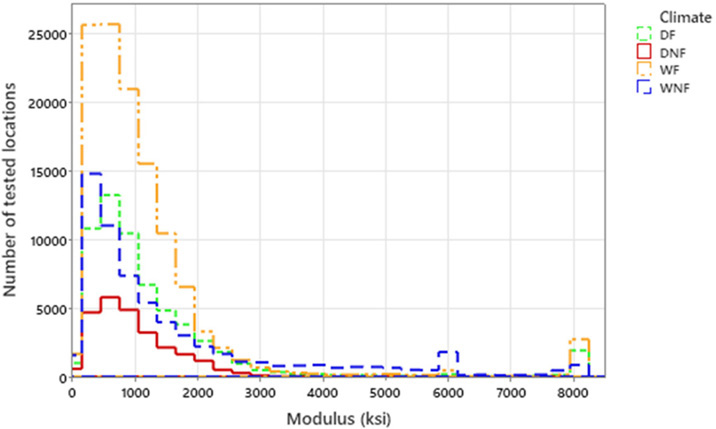
While most of the deflection values and deflection basin parameters were statistically consistent (i.e., a normalized standard deviation between -2.0 and 2.0), the backcalculated modulus values were more likely to vary between consecutive measurements. Figure 32 shows the asphalt layer modulus varied from approximately 100,000 and 8,000,000 psi over the entire testing period. The majority of the backcalculated asphalt layer moduli were between 100,000 and 2,000,000 psi; however, the high layer moduli values were obtained during colder winter days in the northern SMP sections (i.e., Minnesota, Manitoba, Ontario, and Quebec).
Identifying Outliers
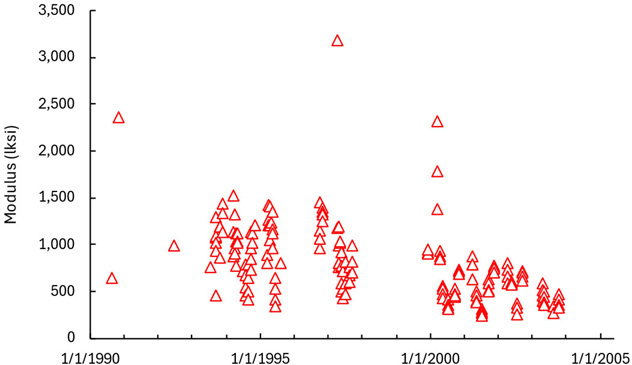
If a discrete limit is used to identify outliers, a significant amount of meaningful data would be eliminated. For example, Figure 33 presents the backcalculated asphalt layer moduli at different dates for Section 27-6251 (Minnesota). As would be expected for this section, the seasonal variation significantly affects the backcalculated modulus. During winter, the asphalt layer modulus reached values as high as 2,000,000 psi and during the thawing season, the modulus dropped as low as 250,000 psi.
To effectively identify the layer moduli outliers, the normalized standard deviation (z-score) was calculated for the asphalt layer modulus. Because the asphalt layer modulus varies hourly, daily, and seasonally, consecutive measurements taken within proximity using the same LTPP data collection method were grouped, and the average of that group was used to identify outliers using:
| (Eq. 47) |
where,
| Z = | z-score of the sample data |
| = | average layer modulus |
| s = | standard deviation of layer modulus |
Asphalt layer moduli with a z-score outside of the range of -2.5 to 2.5 (99% probability assuming normal distribution) were identified as outliers. In addition, if the asphalt layer modulus z-score was rejected, the corresponding layer moduli for the remaining layers was also rejected.
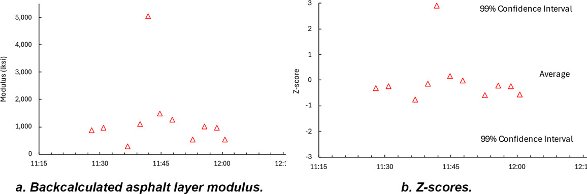
As an example, Figure 34 illustrates the outlier identification process for the asphalt layer modulus for Section 27-6251. FWD testing was performed on March 19, 1997, between 11:30 a.m. and noon. The average modulus was 1,282,000 psi with a standard deviation of 1,299,000 psi. Even though most points did not vary statistically from the average, the backcalculated value at 11:42 a.m. was considerably higher than all other values. The z-score was calculated for each point and shows the test at 11:42 a.m. results in a z-score of 2.92, above the 99% confidence interval (Figure 34). From this analysis, the 11:42 a.m. test was considered an outlier and was removed from further analysis.
A total of 966,320 points were retrieved from all asphalt sections with an FWD testing load of approximately 9,000 lbs and located in the outer wheel path. Table 29 summarizes the total number of FWD tests and identified outliers per climatic zone.
Table 29. Number of FWD Tests and Outliers per Climatic Zone
| Criteria | DF | WF | DNF | WNF | Total |
|---|---|---|---|---|---|
| No. of FWD tests | 229,631 | 402,040 | 91,711 | 242,938 | 966,320 |
| No. of FWD test outliers | 35,919 | 76,986 | 6,327 | 54,171 | 173,403 |
| % FWD tests excluded | 15.6% | 19.1% | 6.9% | 22.3% | 17.9% |
While it is challenging to access the exact causes of FWD test outliers, the presence of structural distress, material properties, and FWD equipment variability can influence the measurements.
Repeatability
FWD measurements were repeated (three to five drops taking just several minutes per test) at each location. Since the temperature and moisture conditions can be considered identical during a short period of time, these measurements should produce highly repeatable results. A satisfactory level of repeatability depends primarily on the FWD load cell and deflection sensor calibration. Rocha et al. (2001) determined equipment calibration can significantly reduce the variability between repeated measurements and showed
calibration, per SHRP guidelines, resulted in all FWD sensors having a coefficient of variation (COV) below 2%.
The number of repeated FWD measurements with the same date, location, and testing time, and 9,000 lb load was 58,043. The average, standard deviation, and COV were calculated for each deflection sensor. Figure 35 illustrates the COV and the 95% confidence interval at each FWD sensor for all climatic zones. In general, the average COV for all climatic zones at each sensor did not surpass 2%. The average value for the center deflection (D1) was approximately 0.5% and steadily increased to approximately 2% for the deflection furthest from the load (D7). However, the D6 sensor had a maximum COV closer to 3% and escalated to 5% for D7. The average COV by sensor for each SMP section is provided in Appendix B.
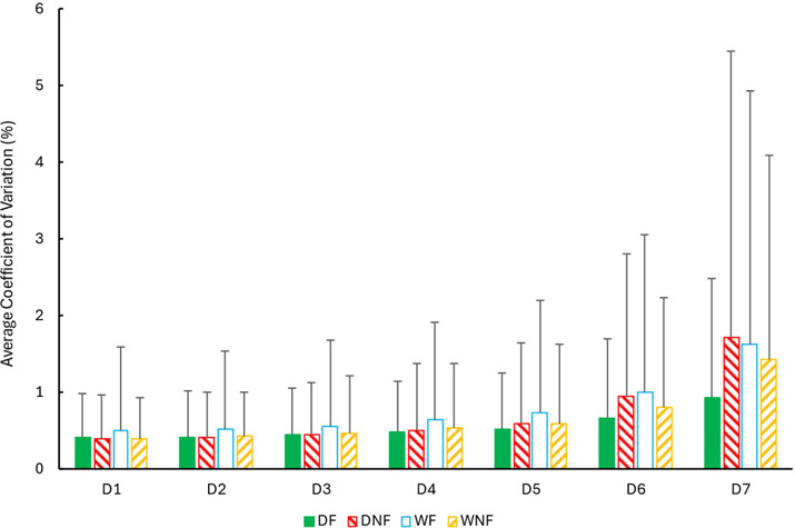
Although the range of sensor variation may seem high, it represents the average repeatability of all FWDs used within the same climate region. It is important to remember the LTPP study was conducted using different FWD brands and models. In addition, COV may not be proportional for all sensors within a single measurement (e.g., COV of D1 is high but attenuates in the farthest sensors from the load or vice versa). However, as the average is calculated per each sensor, those differences were not seen.
Comparisons of Daily Measurements
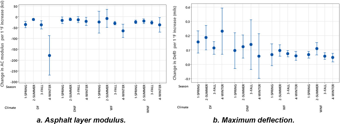
Linear regression models were developed to describe the relationships between the surface temperature and the asphalt layer modulus, maximum deflection, and the calculated deflection basin parameters, resulting in 248 regression models (62 SMP sections, four seasons each). The slope of each regression was then averaged for each season and climatic zone to account for a 1°F change in temperature. Figure 36 illustrates the change in asphalt layer modulus and maximum deflection as a function of temperature. On average, for all climatic zones and seasons, the asphalt layer modulus decreases by 35,000 psi, and the maximum deflection increases by 0.11 mils per 1°F increase in surface temperature.
Influencing Factors
A correlation was conducted to identify environmental and pavement structure factors influencing FWD deflection measurements. FWD deflection measurements were the dependent variables. Independent variables included environmental factors (base and subgrade moisture content, air temperature, pavement temperature, rainfall, 7 days before FWD testing, water table depth) and climatic zone. Pavement structural factors including pavement type, asphalt surface layer thickness, total thickness, and pavement condition were also independent variables.
Environmental Factors
Base and Subgrade Moisture Content
The TDR probes were placed at specified depths based on the sublayer type and thickness (Figure 37). If the top granular base (or subbase) layer was greater than 12 in. thick, the first TDR probe was placed 6 in. below the surface layer and/or bottom of the lowest stabilized layer; otherwise, the probe was placed at mid-depth of the top granular base (or subbase) layer. The next seven TDR probes were placed at 6 in. intervals and the last two probes were placed at 12 in. intervals. Table 30 provides a summary of the TDR moisture content for all SMP sections.
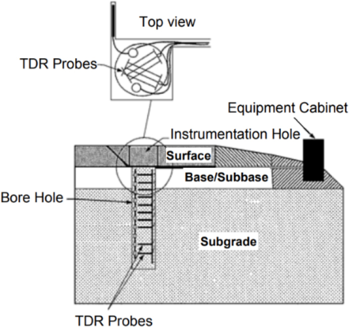
Table 30. TDR Moisture Content Statistical Summary
| TDR No. | No. of Measurements | Minimum (%) | Maximum | Median | Mean | Std Dev |
|---|---|---|---|---|---|---|
| 1 | 4,171 | 0.0 | 43.9 | 13.4 | 14.4 | 6.9 |
| 2 | 3,905 | 0.0 | 47.2 | 14.5 | 15.2 | 8.5 |
| 3 | 3,920 | 1.9 | 50.6 | 17.6 | 18.7 | 9.8 |
| 4 | 3,688 | 0.3 | 48.5 | 16.7 | 19.6 | 10.4 |
| 5 | 3,636 | 0.2 | 45.7 | 18.5 | 20.8 | 10.9 |
| 6 | 3,744 | 0.3 | 48.1 | 20.0 | 24.2 | 11.2 |
| 7 | 3,443 | 0.9 | 47.6 | 21.4 | 24.4 | 11.5 |
| 8 | 3,660 | 0.5 | 53.6 | 22.9 | 26.3 | 12.4 |
| 9 | 3,435 | 0.0 | 54.5 | 23.8 | 25.8 | 12.6 |
| 10 | 3,668 | 0.0 | 54.5 | 26.2 | 28.1 | 12.2 |
Air and Pavement Temperature
Pavement temperature was measured at two locations, about 3 ft from either end of the pavement section. Holes were drilled in the pavement to depths of 1 in. below the surface, at mid-depth, and 1 in. above the bottom of the asphalt or concrete layer. In composite sections, holes were drilled to the same three depths as in concrete, and two additional holes were drilled 1 in. from the top and bottom of the asphalt layer. A summary of measured air and pavement layer temperature for all SMP sections is provided in Table 31.
Table 31. Air and Pavement Layer Temperature Statistical Summary
| Measure | No. of Measurements | Minimum (°F) | Maximum (°F) | Median (°F) | Mean (°F) | Std Dev (°F) |
|---|---|---|---|---|---|---|
| Air | 69,070 | -34.6 | 103.6 | 53.1 | 51.0 | 21.3 |
| Layer 1 | 22,018 | -13.4 | 145.2 | 72.5 | 73.2 | 22.4 |
| Layer 2 | 21,939 | -14.3 | 127.6 | 68.2 | 68.5 | 20.8 |
| Layer 3 | 21,326 | -14.1 | 121.46 | 65.8 | 65.7 | 19.4 |
Rainfall
The statistical summary for rainfall, 7 days before FWD testing, for all SMP sections is summarized in Table 32.
Table 32. Rainfall 7 Days before FWD Testing Statistical Summary
| No. of Measurements | Minimum (in.) | Maximum(in.) | Median (in.) | Mean (in.) | Std Dev (in.) |
|---|---|---|---|---|---|
| 40,652 | 0 | 5.6 | 0.2 | 0.5 | 0.7 |
Water Table Depth
There are 48 SMP sections with water table depth data. The statistical summary of water table depth is summarized in Table 33.
Table 33. Water Table Depth Statistical Summary
| No. of Measurements | Minimum (ft) | Maximum (ft) | Median (ft) | Mean (ft) | Std Dev (ft) |
|---|---|---|---|---|---|
| 1,533 | 0 | 15.8 | 8.0 | 8.2 | 3.2 |
Pavement Structural Factors
Layer Thickness
The asphalt layer could include the original surface layer, overlay, seal coat, asphalt layer below the surface layer, and other surface treatments. In this project, the asphalt layer thickness was calculated as the sum of all asphalt layers in the pavement structure. The median of the asphalt layer thickness was 8.5 in. for all SMP sections; therefore, the asphalt pavement structure was classified as “Thick (H)” ≥ 8.5 in. or “Thin (L)” < 8.5 in. The majority of the SMP sections had an asphalt layer thickness of 5 to 10 in.
The total thickness of a pavement structure is the sum of the thickness of the surface layer, base, and subbase. The median of the total pavement structure thickness was 25 in. for all SMP sections; therefore, the pavement structures were classified as “Thick (H)” ≥ 25 in. or “Thin (L)” < 25 in. The average total thickness of all SMP sections varied from 8.2 to 85.5 in. The majority of SMP sections had a total pavement thickness ranging from 10 to 30 in. The statistical summary of the asphalt layer and total pavement thickness is summarized in Table 34 (details are provided in Appendix B).
Table 34. Asphalt Layer and Total Pavement Thickness Statistical Summary
| Measure | No. of Measurements | Minimum (in.) | Maximum (in.) | Median (in.) | Mean (in.) | Std Dev (in.) |
|---|---|---|---|---|---|---|
| Asphalt Layer | 63 | 2.7 | 21.9 | 8.5 | 9.6 | 4.6 |
| Total Structure | 85 | 8.2 | 85.5 | 24.8 | 28.0 | 15.4 |
Pavement Condition
The Pavement Structural Condition (PSC), developed by the Washington State DOT, was used to assess overall pavement condition at each SMP section based on distress type and severity. The PSC is a single index value used to quantify alligator (fatigue) cracking, longitudinal cracking, transverse cracking, and
patching for asphalt pavements; and slab cracking, joint and crack spalling, pumping, faulting, scaling, and patching for concrete pavements (Kay et al. 1993). The general form of the PSC equation is:
| (Eq. 48) |
where,
| PSC = | pavement structural condition |
| C = | model constant for maximum rating (~100) |
| m = | slope coefficient |
| A = | age since construction or the last resurfacing (years) |
| P = | “selected” constant controlling the degree of curvature of the performance curve |
In total, there were 875 asphalt pavement distress records. Slightly less than half of the records indicated the asphalt pavement was in excellent condition, and the remaining records indicated roughly equal distributions of fair, good, and poor distress conditions. The statistical summary of the PSC for all SMP sections is summarized in Table 35 (details are provided in Appendix B).
Table 35. PSC Statistical Summary
| Measure | Range | No. of Measurements | Probability |
|---|---|---|---|
| Excellent | 75 < PSC ≤ 100 | 407 | 0.47 |
| Good | 50 < PSC ≤ 75 | 182 | 0.21 |
| Fair | 25 < PSC ≤ 50 | 135 | 0.15 |
| Poor | 0 ≤ PSC ≤ 25 | 151 | 0.17 |
FWD Deflections
For the LTPP SMP sections, multiple FWD passes were made to allow for the determination of diurnal effects on deflection measurements. For each pass, it was desired to have 11 FWD runs, beginning at station 0+000.0 (0’) and ending at station 0+152.4 (500 ft) with testing on 50 ft intervals.
Under identical environmental conditions, deflection variations could occur when the load-normalized peak deflections for repeat FWD drops vary by more than the LTPP-specified range of loading. A common cause of the FWD measurement error is uneven pavement surface conditions that result in poor seating of the load plate or deflection sensors. It can also be caused by vibrations from nearby heavy equipment, such as trucks traveling in the adjacent lanes. Under normal conditions, the tolerance range for repeating deflection measurements should fall within the following acceptable range (Schmalzer 2006):
| (Eq. 49) |
where,
| x = | average normalized deflection (mils) of a geophone for all drops at that height |
If temperature and moisture variation during FWD testing had no impact on deflection measurements, the deflections of each of the geophone sensors measured from multiple FWD passes in a single day at one section should fall within the allowable deflection ranges. If the measurements of one sensor exceed the range, it may be concluded that diurnal impacts exist, and temperature adjustment should be applied.
Figure 38 illustrates the number of tests for all locations with at least four FWD runs on a single day as well as the number of tests within and exceeding the LTPP allowable range. The number of tests greater
than the LTPP allowable ranges decreased from D1 to D6, indicating the diurnal temperature effects may need to be considered.

A statistical summary of deflection measurements and deflection basin parameters for all SMP sections is provided in Table 36 (details are provided in Appendix B).
Table 36. FWD-Measured Deflections and Deflection Basin Parameters Statistical Summary
| Measure | No. of Measurements | Minimum | Maximum | Median | Mean | Std Dev |
|---|---|---|---|---|---|---|
| D1 (mils) | 55,768 | 0.5 | 50.2 | 9.64 | 11.14 | 6.4 |
| D2 (mils) | 55,869 | 0.4 | 41.8 | 7.9 | 8.8 | 4.7 |
| D3 (mils) | 55,869 | 0.4 | 29.5 | 6.8 | 7.4 | 3.6 |
| D4 (mils) | 55,869 | 0.3 | 21.5 | 5.4 | 5.7 | 2.6 |
| D5 (mils) | 55,869 | 0.3 | 16.3 | 4.3 | 4.5 | 2.0 |
| D6 (mils) | 55,869 | 0.3 | 12.0 | 2.8 | 2.9 | 1.3 |
| SCI (mils) | 55,768 | 0.0 | 29.9 | 2.7 | 3.8 | 3.2 |
| BDI (mils) | 55,869 | 0.0 | 15.1 | 2.4 | 2.9 | 2.0 |
| BCI (mils) | 55,722 | 0.0 | 8.0 | 1.5 | 1.6 | 0.8 |
| DR1 | 17,190 | 0.0 | 0.8 | 0.2 | 0.2 | 0.1 |
| DR2 | 55,768 | 0.2 | 1.0 | 0.7 | 0.7 | 0.1 |
| DR4 | 55,768 | 0.0 | 1.0 | 0.5 | 0.5 | 0.1 |
| F1 | 55,768 | 0.0 | 4.5 | 0.8 | 0.9 | 0.4 |
| AREA | 55,621 | 9.5 | 34.4 | 21.6 | 21.6 | 3.8 |
Temperature and Moisture Adjustments
Using the influencing factors, temperature and moisture adjustments were determined for FWD-measured deflections. Due to the challenges in obtaining moisture measurements, the approach used in the adjustment development included determining (1) adjustments to a standardized deflection (68°F) and (2) adjustments to moisture based on standardized deflections. In this regard, agencies can adjust deflections based on temperature, and where applicable, the adjusted deflections and layer moduli can be further adjusted based on moisture. The FWD adjustment was based on the following assumptions:
- Deflections vary by temperature within a given day and the moisture conditions of the underlying layers are constant over the day of FWD testing.
- Standardized deflections (68°) vary with seasonal moisture variation.
Temperature Adjustment
As described in Chapter 2, significant previous work was available regarding temperature correction of FWD measurements. Temperature corrections were applied to the raw deflections (or layer moduli) using:
| (Eq. 50) |
where,
| D = | measured deflection (mils) |
| K0 = | adjusted deflection to 68°F (mils) |
| K1 = | temperature adjustment factor |
| T = | asphalt layer mid-depth pavement temperature at time of testing (°F) |
A stepwise variable selection method using the minimum Akaike Information Criterion (AIC) and the LogWorth statistic was used to identify statistically significant variables for the K1 model (Sutherland et al. 2023). A hierarchical significance level was used to quantify the importance of each factor (Table 37).
Table 37. Hierarchical Significance Levels
| Most Important | Important | Statistically Significant | Less Statistically Significant | Not Statistically Significant |
|---|---|---|---|---|
| ρ ≤ 0.001 | > 0.001 ρ ≤ 0.01 | > 0.01 ρ ≤ 0.05 | > 0.05 ρ ≤ 0.01 | ρ > 0.1 |
The results of this analysis indicated asphalt layer thickness, climatic zone, and PSC were statistically significant variables for most of the deflection sensors (Table 38).
Table 38. Variable Selection for Temperature Adjustment of Deflections
| Factor | DI | D2 | D3 | D4 | D5 | D6 |
|---|---|---|---|---|---|---|
| Asphalt layer thickness | ||||||
| Climatic zone | ||||||
| Layer 2 temperature | ||||||
| PSC | ||||||
| Rainfall, 7 days before FWD testing | ||||||
| Total thickness |
Note: ![]() most important;
most important; ![]() important;
important; ![]() statistically significant;
statistically significant; ![]() less statistically significant; and
less statistically significant; and ![]() not statistically significant.
not statistically significant.
K1 for adjusting a standardized D1 deflection (at 68°F) to temperature can be expressed as:
| (Eq. 51) |
where,
| K1(T) = | temperature adjustment factor for deflection |
| ßi = | regression coefficients (see Table 39) |
Table 39. ßi Coefficients for Temperature Adjustment of Deflections
| ßi | Description | Value |
|---|---|---|
| 0 | Regression analysis intercept value | -0.0089 |
| 1 | Asphalt layer thickness | < 8.5 in.: 0; ≥ 8.5 in.: -0.0007 |
| 2 | Pavement condition | Poor: 0; Fair: 0.0033; Good: -0.0013: Excellent: -0.0025 |
| 3 | Climatic zone | DNF: 0; DF: -0.0009; WF: -0.0012; WNF: 0.0020 |
Moisture Adjustment
The average moisture was calculated for the base layer, the subgrade layer, and the deep subgrade layer. Since the placement of TDR probes was not at the same depths for all SMP sections, Python codes were developed and used to automatically determine which layer the TDR moisture was being measured.
The minimum AIC and regression analysis were used to identify the statistically significant variables for moisture adjustment of FWD-measured deflections. The most significant factors, by deflection sensor, included climatic zone, rainfall 7 days before FWD testing, and average subgrade moisture (Table 40). The statistical results are provided in Appendix J.
Table 40. Variable Selection for Moisture Adjustment of Deflections
| Factor | DI | D2 | D3 | D4 | D5 | D6 |
|---|---|---|---|---|---|---|
| Average base moisture | ||||||
| Average deep subgrade moisture | ||||||
| Average subgrade moisture | ||||||
| Climatic zone | ||||||
| Rainfall, 7 days before FWD testing |
Note: ![]() most important;
most important; ![]() important;
important; ![]() statistically significant;
statistically significant; ![]() less statistically significant;
less statistically significant; ![]() not statistically significant.
not statistically significant.
The K1 factor to adjusting the standardized deflections (at 68°F) for moisture can be expressed as:
| (Eq. 52) |
where,
| K1(m) = | moisture adjustment factor for deflection |
| ßi = | regression intercept value (see Table 41) |
Table 41. ßi Coefficients for Moisture Adjustment of Deflections
| ßi | Description | Value |
|---|---|---|
| 0 | Regression analysis intercept value | 2.1714 |
| 1 | Climatic zone | DNF: 0; DF: 0.2769; WF: 0.0822; WNF: -0.0371 |
| 2 | Rainfall, 7 days before FWD testing | 0.0493 |
| 3 | Average subgrade moisture | 0.0225 |
Case Example: Arizona SMP 04-0113
The regression models developed as part of this project are based on relatively limited and geographically spaced data (i.e., 85 SMP sections, 38 agencies, 18 agencies with more than 1 SMP section). While this case example illustrates the application of the research findings, model prediction will be greatly improved when developed from a dataset specific to local conditions.
SMP Section 04-0113 is in Arizona, on Highway 93, approximately 20 miles northeast of Kingman, Arizona. The highway is classified as a rural principal arterial and is in the DNF climatic zone. The pavement structure consisted of a thin asphalt layer, an unbound base layer, and sand with silt and gravel subgrade (Figure 39).

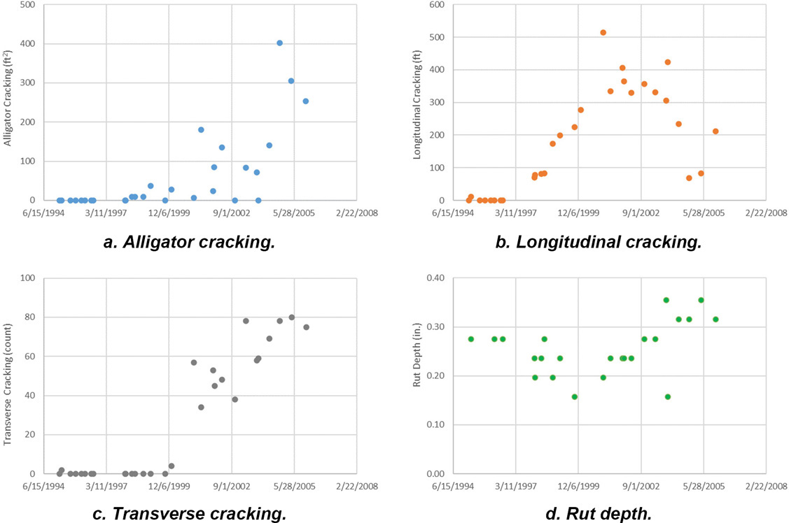
The pavement condition, over the performance period, is shown in Figure 40. Over the performance period, the maximum amount of alligator cracking was approximately 400 ft2 (~12% of wheel path area), longitudinal cracking was less than 550 ft, transverse cracking was less than 80 cracks (about one every 6 ft), and rutting was less than 0.40 in.
The following step-by-step process is used to apply temperature adjustments to the measured D1 deflection.
Step 1. Identify Factors for Analysis
As described previously, the most statistically significant influencing factors for adjusting deflections for temperature on asphalt pavements include pavement condition, asphalt layer thickness, and climatic zone. For this case example, the asphalt layer thickness was categorized as “thin.” There was very little noted pavement distress in December 1995; therefore, the pavement condition was characterized as “excellent.”
Step 2. Determine Deflection Adjustment to Standard Temperature and K0
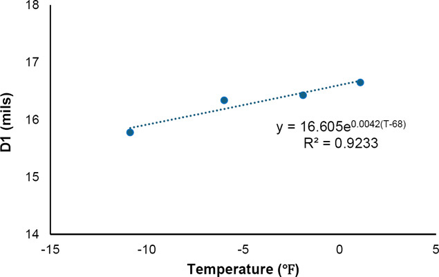
Determine the regression equation to adjust measured deflections to a standard deflection at 68°F by associating the maximum deflection (D1) and the mid-depth asphalt temperature at the time of FWD testing. K0 is determined from the determined regression equation.
The regression equation can be established, for example, via spreadsheet application, developed macro, or statistical software. For example, the regression equation for the measured deflection (D1) at Station 155 is shown in Figure 41 and the resulting K0 is 16.605 mils.
Step 3. Determine Predicted Deflection
Based on the information provided in Steps 1 and 2 (i.e., thin asphalt layer thickness, excellent pavement condition, DNF climatic zone, and K0), the K1 at Station 155 is:
| (Eq. 53) |
The temperature-adjusted deflection at D1 is summarized in Table 42.
Table 42. Adjusted Deflections (Section 04-0113)
| Station | Measured D1 (mils) | Temperature (°F) | K0 | Adjusted D1 (mils) | Relative Error (%) |
|---|---|---|---|---|---|
| 91 | 7.33 | 55.76 | 7.518 | 8.64 | 17.9% |
| 7.34 | 60.60 | 8.18 | 11.4% | ||
| 7.52 | 64.29 | 7.84 | 4.3% | ||
| 7.51 | 68.74 | 7.46 | -0.7% | ||
| 99 | 9.51 | 55.90 | 9.964 | 11.44 | 20.3% |
| 9.67 | 60.78 | 10.82 | 11.9% | ||
| 9.88 | 64.53 | 10.37 | 4.9% | ||
| 9.97 | 68.77 | 9.88 | -0.9% | ||
| 107 | 8.78 | 56.01 | 9.369 | 10.74 | 22.3% |
| 9.04 | 60.94 | 10.15 | 12.3% | ||
| 9.21 | 64.67 | 9.73 | 5.7% | ||
| 9.40 | 68.81 | 9.28 | -1.2% | ||
| 114 | 8.47 | 56.14 | 9.174 | 10.50 | 24.0% |
| 8.80 | 61.12 | 9.92 | 12.8% | ||
| 8.90 | 64.90 | 9.50 | 6.8% | ||
| 9.27 | 68.85 | 9.09 | -2.0% | ||
| 122 | 7.00 | 56.28 | 7.269 | 8.31 | 18.7% |
| 7.12 | 61.23 | 7.85 | 10.3% | ||
| 7.18 | 65.05 | 7.52 | 4.7% | ||
| 7.30 | 68.88 | 7.20 | -1.4% | ||
| 130 | 8.36 | 56.43 | 8.973 | 10.24 | 22.5% |
| 8.62 | 61.39 | 9.67 | 12.2% | ||
| 9.00 | 65.28 | 9.26 | 2.8% | ||
| 8.91 | 68.92 | 8.88 | -0.3% | ||
| 137 | 14.61 | 56.57 | 15.909 | 18.12 | 24.0% |
| 15.01 | 61.57 | 17.12 | 14.0% | ||
| 15.35 | 65.50 | 16.37 | 6.6% | ||
| 15.83 | 68.97 | 15.73 | -0.6% | ||
| 145 | 14.34 | 56.86 | 15.236 | 17.30 | 20.6% |
| 14.70 | 61.68 | 16.37 | 11.4% | ||
| 14.95 | 65.66 | 15.65 | 4.7% | ||
| 15.39 | 69.01 | 15.06 | -2.1% | ||
| 152 | 16.91 | 57.00 | 17.023 | 19.30 | 14.1% |
| 16.89 | 61.86 | 18.26 | 8.1% | ||
| 17.05 | 65.88 | 17.44 | 2.3% | ||
| 17.02 | 69.04 | 16.82 | -1.2% |


