Unknown Quantity: A Real and Imaginary History of Algebra (2006)
Chapter: 9 An Oblong Arrangement of Terms
Chapter 9
AN OBLONG ARRANGEMENT OF TERMS
§9.1 HERE IS A WORD PROBLEM. I found the problem easier to visualize if I thought of the three different kinds of grain as being different colors: red, blue, and green, for instance.
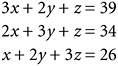
Problem. There are three types of grain. Three baskets of the first, two of the second, and one of the third weigh 39 measures. Two baskets of the first, three of the second, and one of the third weigh 34 measures. And one basket of the first, two of the second, and three of the third weigh 26 measures. How many measures of grain are contained in one basket of each type?
Let’s suppose that one basket of red grain contains x measures by weight, one basket of blue grain contains y measures, and one basket of green grain contains z measures. Then I have to solve the following system of simultaneous linear equations for x, y, and z:
The solution, as you can easily check, is ![]() ,
, ![]() ,
, ![]() .
.
Neither Diophantus nor the mathematicians of Old Babylon would have had much trouble with this problem. The reason it has such a prominent place in the history of mathematics is that the writer who posed it developed a systematic method for solving this and any similar problem, in any number of unknowns—a method that is still taught to beginning students of matrix algebra today. And all this took place over 2,000 years ago!
We do not know that mathematician’s name. He was the author, or compiler, of a book titled Nine Chapters on the Art of Calculation. A collection of 246 problems in measurement and calculation, this was far and away the most influential work of ancient Chinese mathematics. Its precise influence on the development of medieval Indian, Persian, Muslim, and European mathematics is much debated, but versions of the book circulated all over East Asia from the early centuries CE onward, and given what we know of trade and intellectual contacts across Eurasia in the Middle Ages, it would be astonishing if some West-Asian and Western mathematics did not draw inspiration from it.
From internal evidence and some comments by the editors of later versions, we can place the original text of Nine Chapters in the former Han dynasty, which lasted from 202 BCE to 9 CE. This was one of the great epochs of Chinese history, the first in which the empire covered most of present-day metropolitan China,87 and was securely unified under confident native rulers.
The Chinese culture area had actually been unified earlier by the famous and terrible “First Emperor” under his Qin dynasty in 221 BCE. After that tyrant died 11 years later, however, the Qin political system quickly fell apart. Years of civil war followed (providing China with a wealth of themes for literature, drama, and opera) before one of the warlords, a man named Liu Bang, obtained supremacy over his rivals and founded the Han dynasty in 202 BCE.
One of the Qin tyrant’s most notorious deeds was the burning of the books. In accordance with the strict totalitarian doctrines of a philosopher named Shang Yang, Qin had ordered all books of specu-
lative philosophy to be handed in to the authorities for burning. Fortunately, learning in ancient China was done mainly by rote memorization,88 so after the Qin power collapsed, scholars with the destroyed texts still in their heads could reproduce them. Possibly this was the point when the Nine Chapters took decisive form, as a unified compilation of remembered texts from one or many sources. Or possibly not: The tyrant’s edict exempted books on agriculture and other practical subjects, so that if the Nine Chapters existed earlier than the Han, it would not likely have been burned.
At any rate, the Early Han dynasty was a period of mathematical creativity in China. Peace brought trade, which demanded some computational skills. The standardization of weights and measures, begun by the Qin, led to an interest in the calculation of areas and volumes. The establishment of Confucianism as the foundation for state dogma required a reliable calendar so that the proper observances could be carried out at proper times. A calendar was duly produced, based on the usual 19-year cycle.89
Nine Chapters was probably one fruit of this spell of creativity. The book certainly existed by the 1st century CE and played a part in the subsequent mathematical culture of China comparable to that played by Euclid’s Elements in Europe. And there, in the eighth chapter, is the grain measurement problem I described.
How does the author of Nine Chapters solve the problem? First, multiply the second of those equations by 3 (which will change it to 6x + 9y + 3z = 102); then subtract the first equation from it twice. Similarly, multiply the third equation by 3 (making it 3x + 6y + 9z = 78) and subtract the first equation from it once. The set of three equations has now been transformed into this:
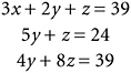
Now multiply that third equation by 5 (making it 20y + 40z = 195) and subtract the second equation from it four times. That
third equation is thereby reduced to
from which it follows that ![]() . Substituting this into the second equation gives the solution for y, and substituting the values of z and y into the first equation gives x.
. Substituting this into the second equation gives the solution for y, and substituting the values of z and y into the first equation gives x.
This method is, as I said, a very general one, which can be applied not just to three equations in three unknowns but to four equations in four unknowns, five equations in five unknowns, and so on.
The method is known nowadays as Gaussian elimination. The great Carl Friedrich Gauss made some observations of the asteroid Pallas between 1803 and 1809 and calculated the object’s orbit. This involved solving a system of six linear equations for six unknowns. Gauss tackled the problem just as I did above—which is to say, just as the unknown author of Nine Chapters on the Art of Calculation had 2,000 years previously.
§9.2 Once we have a good literal symbolism to hand, it is natural to wonder what solutions we would get for x, y, and z if we were to slog through the Gaussian elimination method for a general system of three equations, like this one:
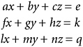
Here is the result:
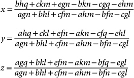
That is the kind of thing that makes people give up math. If you persevere with it, though, you begin to spot some patterns among the spaghetti. The three denominators, for instance, are identical.
Let’s concentrate on that denominator, the expression agn + bhl + cfm − ahm − bfn − cgl. Note that e, k, and q don’t show up in it at all. It’s constructed entirely from the coefficients at the left of the equals signs—that is, from this array:

Next thing to notice: None of the six terms in that expression for the denominator contain two numbers from the same row of the array or two from the same column.
Look at the ahm term, for instance. Having picked a from the first row, first column, it’s as if the first row and the first column are now out of bounds. The next number, h, can’t be taken from them; it has to be taken from elsewhere. And then, having taken h from the second row, third column, that row and column are then out of bounds, too, and there is no choice but to take m from the third row, second column.
It is not hard to show that applying this logic to a 3 × 3 array gives you six possible terms. For a 2 × 2 array, you would get two terms; for a 4 × 4 array, 24 terms. These are the factorial numbers I introduced in §7.4:2! = 2, 3! = 6, 4! = 24. The corresponding number of terms for five equations in five unknowns would be 5!, which is 120.
The signs of the terms are more troublesome. Half are positive and half negative, but what determines this? Why is the agn term signed positive but ahm negative? Watch carefully.
First note that I was careful to write my terms, like that ahm, with the letters in order by the row I took them from: a from row 1, h from row 2, m from row 3. Then a term can be completely and unambiguously described by the columns the letters come from, in this case columns 1, 3, and 2. The quartet (1, 3, 2) is a sort of alias for ahm, so
long as I stick to my principle of writing the coefficients in row order, which I promise to do.
It is also, of course, a permutation of the basic triplet (1, 2, 3), the permutation you get if you replace the basic 2 by 3 and the basic 3 by 2.
Now, permutations come in two varieties, odd and even. This particular permutation is odd, and that is why ahm has a minus sign in front. The term bhl, on the other hand, has the alias (2, 3, 1), as you can easily check. This is the permutation you get to from basic (1, 2, 3) if you replace 1 by 2, 2 by 3, and 3 by 1. It is an even permutation, and so bhl has a plus sign.
Wonderful, but how do you tell whether a permutation is odd or even? Here’s how. I’ll continue using the expression for three equations with three unknowns, but all of this extends easily and obviously to 4, 5, or any other number of equations.
Form the product (3 − 2) × (3 − 1) × (2 − 1) using every possible pair of numbers (A − B) for which A > B and A and B are either 1, 2, or 3. The value of this product is 2 (which is 2! × 1!, so you can easily see the generalization. If we were working with four equations in four unknowns, the product would be (4 − 3) × (4 − 2) × (4 − 1) × (3 − 2) × (3 − 1) × (2 − 1), which is 12, which is 3! × 2! × 1!). This value, however, doesn’t actually matter. What matters is its sign, which of course is positive.
Now just walk through that expression applying some permutation to the numbers 1, 2, and 3. Try that first permutation, the one for ahm, where we replace the basic 2 by 3 and 3 by 2. Now the expression looks like (2 − 3) × (2 − 1) × (3 − 1), which works out to −2. So this is an odd permutation. Applying the bhl permutation, on the other hand, changes (3 − 2) × (3 − 1) × (2 − 1) into (1 − 3) × (1 − 2) × (3 − 2), which is +2. This is an even permutation.
This business of even and odd permutations is an important one, obviously related to the issues I discussed in §§7.3-7.4. Here are all six possible permutations of (1, 2, 3), with their parity (even or odd) worked out by the method I just used:
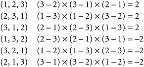
As you can see, half have even parity, half odd. It always works out like this.
So the sign on each term in that denominator expression is determined by the sign of the alias permutation that corresponds to the coefficients. Whew!
The denominator expression I have been working over here is an example of a determinant. So, as a matter of fact, are the numerators I got for x, y, and z. You might try figuring out which 3 × 3 array each numerator is the determinant of. The study of determinants led eventually to the discovery of matrices, now a vastly important subtopic within algebra. A matrix is an array of (usually) numbers, like that 3 × 3 one I set out above but treated as an object in its own right. More on this shortly.
It is an odd thing that while a modern course in algebra introduces matrices first and determinants later, the historical order of discovery was the opposite: determinants were known long before matrices.
The fundamental reason for this, which I shall enlarge on as I go along, is that a determinant is a number. A matrix is not a number. It is a different kind of thing—a different mathematical object. And the period we have reached in this book (though not yet in this chapter, which still has some prior history to fill in) is the early and middle 19th century, when algebraic objects were detaching themselves from the traditional mathematics of number and position and taking on lives of their own.
§9.3 Although mathematicians doodling with systems of simultaneous linear equations must have stumbled on determinant-type expressions many times over the centuries, and some of the algebraists I have already mentioned—notably Cardano and Descartes—came close to discovering the real thing, the actual, clear, indisputable discovery of determinants did not occur until 1683. It is one of the most remarkable coincidences in the history of mathematics that the discovery of determinants took place twice in that year. One of these discoveries occurred in the kingdom of Hanover, now part of Germany; the other was in Edo, now known as Tokyo, Japan.
The German mathematician is of course the one more familiar to us. This was the great Gottfried Wilhelm von Leibniz, co-inventor (with Newton) of the calculus, also philosopher, logician, cosmologist, engineer, legal and religious reformer, and general polymath—“a citizen of the whole world of intellectual inquiry,” as one of his biographers says.90 After some travels in his youth, Leibniz spent the last 40 of his 70 years in service to the Dukes of Hanover, one of the largest of the petty states that then occupied the map of what is now Germany.
In a letter to the French mathematician-aristocrat the Marquis de l’Hôpital, written in that year of 1683, Leibniz said that if this system of simultaneous linear equations—three equations in two unknowns, note—
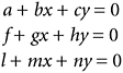
has solutions x and y, then
This is the same as saying that the determinant agn + bhl + cfm − ahm − bfn − cgl must be zero. Leibniz was quite right, and although he did not construct a full theory of determinants, he did understand their importance in solving systems of simultaneous linear equations
and grasped some of the symmetry principles that govern their structure and behavior, principles like those I sketched above.
Leibniz’s Japanese co-discoverer, of whom he lived and died perfectly unaware, was Takakazu Seki, who was born in either 1642 or 1644 in either Huzioka or Edo. “Knowledge of Seki’s life is meager and indirect,” says Akira Kobori in the DSB entry for Seki. His biological father was a samurai, but the Seki family adopted him, and he took their surname.
Japan was at this time a few decades into an era of national unity and confidence under strong rulers—the Edo period, one of whose first and greatest Shoguns was the subject of a colorful novel by James Clavell. Unification and peace had allowed a money economy to develop, so that accountants and comptrollers were in great demand. The patriarch of the Sekis was in this line of work, and Takakazu followed in his footsteps, rising to become chief of the nation’s Bureau of Supply and being promoted to the ranks of samurai himself. “In 1706 [I am quoting from the DSB again] having grown too old to fulfill the duties of his office, he was transferred to a sinecure and died two years later.”
The first math book ever written by a Japanese had appeared in 1622, Sigeyosi Mori’s A Book on Division. Our man Seki was a grand-student of Mori’s—I mean, Seki’s teacher (a man named Takahara, about whom we know next to nothing) was one of Mori’s students. Seki was also strongly influenced by Chinese mathematical texts—no doubt he knew the Nine Chapters on the Art of Calculation.
Seki went far beyond the methods known in East Asia at that time, though, developing a “literal” (the “letters” were actually Chinese characters) symbolism for coefficients, unknowns, and powers of unknowns. Though his solutions for equations were numerical, not strictly algebraic, his investigations went deep, and he came within a whisker of inventing the calculus. What we nowadays call the Bernoulli numbers, introduced to European math by Jacob Bernoulli in 1713, had actually been discovered by Seki 30 years earlier.91
As a samurai, Seki was expected to practice modesty, and that apparently precluded his publishing books in his own name. There was also a culture of secrecy between rival schools of mathematical instruction, rather like the one in 16th-century Italy that I have already described. What we know of Seki’s work is taken from two books published by his students, one in 1674 and one posthumously in 1709. It is in this second book that Seki’s work on determinants appears. He picked up and generalized the Chinese method of elimination by rows, the method that I described earlier, and showed the part played by the determinant in it.
§9.4 Unfortunately, neither Seki’s work nor that of Leibniz had much immediate consequence. There seems to have been no further development in Japan at all until the modern period. In Europe an entire lifetime passed before determinants were taken up again. Then, suddenly, they were “in the air” and by the late 1700s had entered the Western mathematical mainstream.
The process of solving a system of simultaneous linear equations by use of determinants, the process I sketched out in §9.2, is known to mathematicians as Cramer’s rule. It first appeared in a book titled Introduction to the Analysis of Algebraic Curves, published in 1750. The author of the book, Gabriel Cramer, was a Swiss mathematician and engineer, widely traveled and well acquainted with all the great European mathematicians of his day. In his book he tackles the problem of finding the simplest algebraic curve (that is, a curve whose x, y equation has a polynomial on the left of the equals sign and a zero on the right) passing through n arbitrary points in a flat plane. He found that, given an arbitrary five points, we can find a second-degree curve to fit them—a curve, that is, with an equation like this:
I shall have much more to say about this kind of thing later, in my primer on algebraic geometry. Finding the equation of the actual
curve for a given actual five points leads to a system of five simultaneous linear equations in five unknowns. This is not merely an abstract problem. By Kepler’s laws, planets move on curves of the second degree (to a good approximation anyway), so that five observations of a planet’s position suffice to determine its orbit fairly accurately.92
§9.5 Can you make determinants interact with each other? Given two square arrays, for instance, if I were to add their corresponding elements to get a new array, like
is the determinant of that new array the sum of the determinants of the first two? Alas, no: The determinants of the two arrays on the left sum to (ad − bc) + (ps − qr), while the determinant of the array on the right is (a + p) × (d + s) − (b + q) × (c + r). The equality is not true.
While adding determinants doesn’t get you anywhere much, multiplying them does. Let me just multiply those two determinants: (ad − bc) × (ps − qr) is equal to adps + bcqr − adqr − bcps. Is that the determinant of any interesting array? As a matter of fact it is. It is the determinant of this 2 × 2 array:
If you stare hard at that array, you will see that every one of its four elements is gotten by simple arithmetic on a row from the first array—either a, b or c, d—and a column from the second—either p, r or q, s. The element in the second row, first column, for example, comes from the second row of the first array and the first column of the second. This doesn’t just work for 2 × 2 arrays either: If you multiply the determinants of two 3 × 3 arrays, you get an expression which is the determinant of another 3 × 3 array, and the number in the nth
row, mth column of this “product array” is gotten by merging the nth row of the first array with the mth column of the second, in a procedure just like the one described above.93
To a mathematician of the early 19th century, looking at that 2 × 2 product array would bring something else to mind: §159 of Gauss’s great 1801 classic Disquisitiones arithmeticae. Here Gauss asks the following question: Suppose, in some expression for x and y, I make the substitutions x = au + bv, y = cu + dv. In other words, I am changing my unknowns from x and y to u and v by a linear transformation—x a linear expression in u and v, and y likewise. And suppose then I do this substitution business again, switching to yet another couple of unknowns w and z via two more linear transformations: u = pw + qz, v = rw + sz.
What’s the net effect? In going from unknowns x and y to unknowns w and z via those intermediate unknowns u and v, using linear transformations all along the way, what is the substitution I end up with? It’s easy to work out. The net effect is this substitution: x = (ap + br)w + (aq + bs)z, y = (cp + dr)w + (cq + ds)z. Look at the expressions in the parentheses! It seems that multiplying determinants might have something to do with linear transformations.
With these ideas and results floating around, it was only a matter of time before someone established a good coherent theory of determinants. This was done by Cauchy, in a long paper he read to the French Institute in 1812. Cauchy gave a full and systematic description of determinants, their symmetries, and the rules for manipulating them. He also described the multiplication rule I have given here, though of course in much more generality than I have given. Cauchy’s 1812 paper is generally considered the starting point of modern matrix algebra.
§9.6 It took 46 years to get from the manipulation of determinants to a true abstract algebra of matrices. For all the intriguing symmetries and rules of manipulation, determinants are still firmly attached
to the world of numbers. A determinant is a number, though one whose calculation requires us to go through a complicated algebraic expression. A matrix in the modern understanding is not a number. It is an array, like the ones I have been dealing with. The elements stacked in its rows and columns might be numbers (though this is not necessarily the case), and there will be important numbers associated with it—notably its determinant. The matrix, however, is a thing of interest to mathematicians in itself. It is, in short, a new mathematical object.
We can add or subtract two square94 matrices to get another one; we just add the arrays term by term. (This works out to be a suitable procedure for matrices, even though the associated determinants come out wrong.) We can multiply a matrix by an ordinary number to get a different matrix. Does this sound familiar? The family of all n × n matrices forms a vector space, of dimension n2. More than that: We can, using the techniques I illustrated above for determinants, multiply matrices together in a consistent way, so the family of all n × n matrices forms not merely a vector space but an algebra!
We can make a case that this is the most important of all algebras. For example, it encompasses many other algebras. The algebra of complex numbers, to take a simple case, can be matched off precisely—“mapped,” as we say—with all its rules of addition, subtraction, multiplication, and division, to a certain subset of the 2 × 2 matrices. You might care to confirm that the rule for matrix multiplication (it is the same as the one for determinants that I gave in the preceding section) does indeed reproduce complex-number multiplication when complex numbers a + bi and c + di are suitably represented by matrix equivalents:
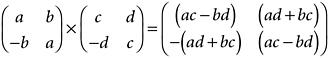
You might want to figure out which matrix represents i in this scheme of things. Then multiply that matrix by itself and confirm that you do indeed get the matrix representing −1.
Hamilton’s quaternions can be similarly mapped into a family of 4 × 4 matrices. The fact of their multiplication not being commutative doesn’t matter, since matrix multiplication is not commutative either (though a particular family of matrices, like the one representing complex numbers, might preserve commutativity within itself). Noncommutativity was cropping up all over mid-19th-century algebra. Permutations, also noncommutative, can be represented by matrices, too, though the math here would take us too far afield.
Matrices are, in short, the bee’s knees. They are tremendously useful, and any modern algebra course quite rightly begins with a good comprehensive introduction to matrices.
§9.7 I said that it took 46 years to get from determinants to matrices. Cauchy’s definitive paper on determinants was read to the French Institute in 1812. The first person to use the word “matrix” in this algebraic context was the English mathematician J. J. Sylvester in a scholarly article published in 1850. Sylvester defined a matrix as “an oblong arrangement of terms.” However, his thinking was still rooted in determinants. The first formal recognition of a matrix as a mathematical object in its own right came in another paper, “Memoir on the Theory of Matrices,” published in the Transactions of the London Philosophical Society by the English mathematician Arthur Cayley in 1858.
Cayley and Sylvester are generally covered together in histories of mathematics, and I see no reason to depart from this tradition. They were near coevals, Sylvester (born 1814) seven years the older. They met in 1850, when both were practicing law in London, and became close friends. Both worked on matrices; both worked on invariants (of which more later). Both studied at Cambridge, though at different colleges.
Cayley was elected a fellow of his college—Trinity, Cambridge—and taught there for four years. To continue, he would have had to take holy orders in the Church of England, which he was not willing
to do. He therefore went into the law, being admitted to the bar in 1849.
Sylvester’s first job was as a professor of natural philosophy at the new University of London. De Morgan (see §10.3) was one of his colleagues. In 1841, however, Sylvester left to take up a professorship at the University of Virginia. That lasted three months; then he resigned after an incident with a student. The incident is variously reported, and I don’t know which report is true. It is clear that the student insulted Sylvester, but the stories differ about what happened next. Sylvester struck the student with a sword-stick and refused to apologize; or Sylvester demanded that the university discipline the student, but the university would not. There is even a theory involving a homoerotic attachment. Sylvester never married, wrote florid poetry, enjoyed singing in a high register, and brought forth the following comment from diarist and mathematical hanger-on Thomas Hirst:
On Monday having received a letter from Sylvester I went to see him at the Athenaeum Club … He was, moreover, excessively friendly, wished we lived together, asked me to go live with him at Woolwich and so forth. In short he was eccentrically affectionate.
Whatever the facts of the case, I don’t think we need to venture into speculations about Sylvester’s inner life to see that the traits of character noted above, together with his Jewishness (he was born with the surname Joseph; “Sylvester” was a later family addition) and his anti-slavery opinions, would not have done much to commend him to the young bloods of antebellum Charlottesville. He returned to England, took a job as an actuary, studied for the bar, and supplemented his income by taking private students (one of whom was Florence Nightingale, “the lady with the lamp,” who was a very capable mathematician and statistician).
Cayley and Sylvester were just two of a fine crop of algebraists that came up in the British Isles in the early 19th century. Hamilton,