This page intentionally left blank.

§FT.1 “FIELD” AND “GROUP” ARE the names of two mathematical objects that were discovered in a series of steps during the early 19th century.

A field is a more complicated thing than a group, so far as its internal structure goes. For this reason, textbooks of algebra usually introduce groups first and then advance to fields, even though there is a sense in which a field is a more commonplace kind of thing than a group and therefore easier to comprehend. Being simpler, groups also have a wider range of applicability, so that on the whole, group theory is more challenging to the pure algebraist than field theory.¹⁰⁶

For these reasons, and also to make Galois’ discoveries more accessible, I am going to describe fields here in this primer, before going into more detail about groups in the chapter that follows.

§FT.2 A field is a system of numbers (or other things—but numbers will serve for the time being) that you can add, subtract, multiply, and divide to your heart’s content. No matter how many of the four basic operations you do, the answer will always be some other

number in the same field. That is why I said that a field is a commonplace sort of thing. When you are in a field, you are doing basic arithmetic: +, −, ×, ÷. If you want a visual mnemonic for the algebraic concept of a field, just imagine the simplest kind of pocket calculator, with its four operation keys: +, −, ×, ÷.

There are certain rules to be followed, none of them very surprising. I have already mentioned the closure rule: Results of arithmetic operations stay within the field. You need a “zero” that leaves other numbers unchanged when you add it and a “one” that leaves them unchanged when you multiply by it. Basic algebraic rules must apply: a × (b + c) always equal to a × b + a × c, for instance. Both addition and multiplication must be commutative; we have no truck with noncommutativity in fields. Hamilton’s quaternions are therefore not a field, only a “division algebra.”

Neither nor is a field, since dividing two whole numbers may not give a whole-number answer. The family of rational numbers does form a field, though. You can add, subtract, multiply, and divide as much as you like without ever leaving . It’s a field. There is a sense in which is the most important, the most basic, field. The real numbers form a field, too. So do the complex numbers , using the rules for addition, subtraction, multiplication, and division that I gave at the beginning of this book. We therefore have three examples of fields already to fix our ideas on: , , and .

Are there any other fields besides , , and ? There certainly are. I am going to describe two common types. Then I shall put the two types together to lead into Galois theory and group theory. Then, as a footnote, I shall mention a third important type of field.

§FT.3 The first other type of field—other than the familiar , , and —is the finite field. , , and all have infinitely large memberships. There is an infinity of rational numbers; there is an infinity of real numbers; and there is an infinity of complex numbers.

Here is a field with only three numbers in it, which for convenience I shall call 0, 1, and 2, though if you find this leads to too much confusion with the more usual integers with those names, feel free to scratch out my 0, 1, 2, and replace them with any other symbols you please: perhaps “Z” for the zero, “I” for the one, and “T” for the third field element. It will not be the case in this field, for example, that 2 + 2 = 4. In this field, 2 + 2 = 1. Here, in fact, are the complete addition and multiplication tables for my sample finite field, whose name is F₃.

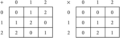
FIGURE FT-1 The field F₃.

Note some points about this field. First, since the additive inverse (“negative”) of 1 is 2, and vice versa, there is not much point in talking about subtraction. “… −1” can always be replaced by “…+ 2,” and vice versa.¹⁰⁷ Same with division. Since the multiplicative inverse (“reciprocal”) of 2 is 2 (because 2 × 2 = 1), a division by 2 can always be replaced by a multiplication by 2, with exactly the same result! Division by 1 is trivial, and division by zero is never allowed in fields.

Is there a finite field for every natural number greater than 1? No. There are finite fields only for prime numbers and their powers. There are finite fields with 2, 4, 8, 16, 32, … members; there are finite fields with 3, 9, 27, 81, 243, … members; and so on. There is, however, no finite field with 6 members or 15 members.

Finite fields are often called Galois fields, in honor of the French mathematician Évariste Galois, whom we shall meet presently in the main text.

§FT.4 The second other type of field is the extension field. What we do here is take some familiar field—very often —and append one extra element to it. The extra element should, of course, be taken from outside the field.

Suppose, for example, we append the element to . Since is not in , this should be just the kind of thing I am talking about. If I now add, subtract, multiply, and divide in this enlarged family of numbers, I get all numbers of the form , where a and b are rational numbers. The sum, difference, product, and quotient of any two numbers of this kind are other numbers of the same kind. The rules for addition, subtraction, multiplication, and division in fact look rather like the rules for complex numbers. Here, for example, is the division rule:

This is a field. I have extended the field of rational numbers by just appending the one irrational number . This gives me a new field.

Note that this new field is not , the field of real numbers. All kinds of real numbers are not in it: , , π, and an infinite host of others. The only numbers that are in it are (i) all the rational numbers, (ii) , and (iii) any number I can get by combining with rational numbers via the four basic arithmetic operations.

Why would I want to go to all this trouble to extend by such a teeny amount? To solve equations, that’s why. The equation x² − 2 = 0

has no solutions in , as Pythagoras discovered to his alarm and distress. In this new, slightly enlarged field, it does have solutions, though: and . By extending fields judiciously, I can solve equations I couldn’t solve before.

Notice an interesting and important thing: The extended field is a vector space over the original field . An example of two linearly independent vectors would be the numbers 1 and . These would, in fact, make an excellent basis (see §VS.3) for the vector space. Every other vector—every number of the form , with a and b both rational—can be expressed in terms of them. Considered in this way, as a vector space, the extended field is two-dimensional.

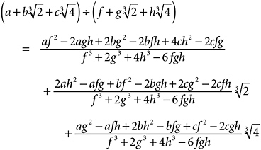
The field you get by appending an irrational number to will not always be two-dimensional. If, for example, you were to append , the extension field would be three-dimensional, with the three vectors 1, , as a suitable basis. Here, just to show how quickly things can get out of control, is the rule for division in this field:

§FT.5 I am now going to put the previous two sections together and solve some quadratic equations in my 0, 1, 2 field. The advantage of finite fields, you see, is that you can write down all possible quadratic equations!

First things first. Here are all possible linear equations in my 0, 1, 2 field, with their solutions, which you can check if you like against the addition and multiplication tables for that field.

In fact, I have even made too much of that. The first two equations are not really interesting. Of course the solution of 2x = 0 is x = 0! A bit less obvious, neither are the last two very interesting. Their left-hand sides factorize to, respectively, 2(x + 2) and 2(x + 1), so they are really just the third and fourth equations over again in light disguise. (Remember that in this field 2 × 2 = 1.) Only the middle two equations are really of any interest.

On to quadratic equations. This time I shall discard the uninteresting ones in advance. Here are all the interesting quadratic equations with coefficients in F₃. For extra points, I have factorized them, too.

An equation that has no solutions in the field I am working with is called irreducible. (Compare Endnote 34.) You can see that of the six interesting equations with coefficients in the 0, 1, 2 field, three are irreducible.

See what I have done? I have re-created in miniature the situation you get with “normal” quadratic equations—except that, instead of an infinity of equations to worry about, in this field there are only six: three with solutions, three irreducible. In normal arithmetic the equation x² − 2 = 0 has no solutions in because is not a rational number. Similarly, the equation x²+ 1 = 0 has no solutions in , or even in , because is not in either or .

§FT.6 Can we extend the 0, 1, 2 field so that those irreducible equations have solutions? Yes, we can. Let’s invent a new number—I shall just call it a—that satisfies that first equation: a² + 1 = 0. Adding 2 to each side, a² = 2. (So you could call a a square root of 2. Since this 2 isn’t really behaving altogether like a regular 2, though, I won’t write a as . I’ll just leave it incognito as a.) And now all the equations can be solved:

We just needed to add that one element a to the field, and we can solve all quadratic equations. And all addition, subtraction, multipli-

cation, and division in the extended field, which is commonly denoted by F₃(a), involve nothing more than linear expressions in a. If a multiplication results in a², you can at once replace it by 2 because a² = 2. Here is the multiplication table for the extended field. (The addition table is less exciting, though you should feel free to construct it if you want to.)

FIGURE FT-2 The multiplication table for F₃(a).

§FT.7 There we have some highly concentrated essence of Galois theory. We have an equation whose coefficients belong to a certain field but whose solutions can’t be found in that field. In order to encompass those solutions, we extend our coefficient field to a larger field—call it the solution field. The issue Galois was concerned with, the issue of what form the solutions of our equation will take, depends on the relationship between these two fields, the coefficient field and the solution field.

That was Galois’ great insight. His discovery was that this relationship can be expressed in the language of group theory, which, in 1830, meant the language of permutations.

Galois found that, for any given equation, we need to consider certain permutations of the solution field. The solution field, like my F₃(a) above, is in general bigger than the coefficient field (F₃ in my example). Now, among all useful permutations of the solution field, there is a subfamily of permutations that leave the coefficient field unchanged. That subfamily forms a group, which we call the Galois group of the equation. All questions about the solvability of the equation translate into questions about the structure of that group.

In the case of the equation I began this section with, the equation x² + 1 = 0, with coefficients understood to be taken from the minifield F₃, the Galois group is a rather simple one, with only two members. One of those members is the identity permutation I, which leaves everything alone. The other is the permutation that exchanges the two solutions, sending a to 2a and 2a to a. This permutation—let’s call it P—acts on the whole of F₃(a), of course. Using an arrow to indicate “permutes to,” it acts like this: 0 → 0, 1 → 1, 2 → 2, a → 2a, 2a → a, 1 + a → 1 + 2a, 1 + 2a → 1 + a, 2 + a → 2 + 2a, 2 + 2a → 2 + a.

Here is a “multiplication” table for the Galois group of the equation x² + 1 = 0 over the coefficient field F₃. Multiplication here means the compounding of permutations—doing one permutation, then doing the other.

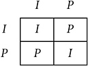
FIGURE FT-3 The multiplication table for the Galois group of x² + 1 = 0.

§FT.8 That is a grossly oversimplified account of Galois theory, of course.¹⁰⁸ It is all very well to speak of permuting things like F₃ or F₃(a), which have only three and nine members, respectively. What had been vexing algebraists for all those centuries was the solution of polynomials with coefficients in , a field with infinitely many members. How do you permute that?

I hope to make this a little clearer as I proceed. I doubt I can make things much clearer, though. Galois theory is a difficult and subtle branch of higher algebra, not easily accessible to the nonmathematician. If you can keep in your mind the fact that a polynomial with coefficients in a certain field may have roots in a bigger field, that the relationship between these two fields, the bigger one and the smaller one, can be expressed in the language of group theory, and that every question about solving a polynomial equation can thereby be translated into a question about group theory, you will have grasped the essence of Galois’s achievement.

§FT.9 Before leaving the topic of fields, I had better add one more type of field, mainly by way of apology. In discussing the work of the 18th-century algebraists, I used the word “polynomial” a bit indiscriminately, just for the sake of simplicity. Some of those usages should really have been not “polynomial” but “rational function.”

A rational function is the ratio of two polynomials, like this:

Since, with a little labor, any two such functions can be added, subtracted, multiplied, or divided, they form a field.

Note that a field of rational functions “depends on” another field, the field from which the coefficients of the polynomials are taken. A field of rational functions can in fact be viewed from the perspective of field extensions, as described above. I start with my coefficient field, whatever it is. Then I append the symbol x and permit all possible

additions, subtractions, multiplications, and divisions. This generates the rational-function field. The only difference between this and my previous examples of field extensions is that in those cases I had a better handle on the thing I was appending. I knew that its square, or its cube, was 2. This allowed me to do a lot of simplification on the field arithmetic. Here I don’t know anything about x. It’s just a symbol—an unknown quantity, if you like….