§AG.1 GEOMETRY, AS I SHALL DESCRIBE in the next chapter, has had a crucial influence on modern algebra. My main text will try to track the nature and growth of that influence. Here I only want to introduce a handful of basic ideas about algebraic geometry. In a fine old mathematical tradition, I shall use conic sections as an introduction to this topic.

§AG.2 Conic sections, often just called “conics,” are a family of plane curves, the ones you get when your plane intersects a circular cone. (And note that a cone, mathematically considered, does not stop at its apex but extends to infinity in both directions.) In Figure AG-1 the intersecting plane is the page you are reading, which you must imagine to be transparent. The apex of the cone lies behind this plane. In the first picture, the cone’s axis is at right angles to the paper, so the intersection is a circle. I then rotate the cone, bringing the further end up. The circle becomes an ellipse. Then, as I tilt the cone up further, one end of the ellipse “goes to infinity,” giving a parabola. Tilting beyond that point gives a two-part curve called a hyperbola.¹²⁸

FIGURE AG-1 Conic sections formed by a cone intersecting this page.

That, of course, is all geometry. To get to algebra, we follow Descartes. For the infinity of points that define a conic, Descartes’ x and y coordinates satisfy a quadratic equation in x and y, like this one:

(The precise choice of letters for the coefficients there—a, h, b, g, f, c—may seem a little eccentric, but I’ll explain that later.) Another way of saying the same thing is: A conic is the zero set of some quadratic polynomial in two unknowns. It is the set of points (x, y) that make the polynomial work out to zero.

The ellipse shown in Figure AG-2a, for example, has the equation

Now suppose I were to move that ellipse to some other part of the plane and rotate it a little while doing so (Figure AG-2b). What happens to its algebraic equation?

The equation has of course changed. The new equation for my ellipse is

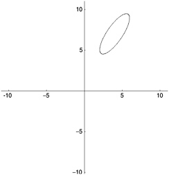
FIGURE AG-2a

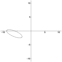
FIGURE AG-2b

However, it’s still the same conic. Its size and shape haven’t changed. It’s not larger or smaller, not rounder or skinnier.

So now the following very interesting question arises: What is there in those two algebraic expressions to tell us that they both refer to the same conic? In passing from one equation to the other, what was left unchanged or, as mathematicians say, invariant?

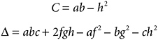
The answer is not obvious. All the coefficients changed in size, and in two cases the sign flipped too (negative to positive). There are invariants hidden in there, though. Writing the general case once again as

compute the following things:

In the two equations for my ellipse, these work out to C = 5625 and 257049, Δ = −1265625 and −390971529. Plainly these aren’t invari-

ants either. But look! Calculate Δ²/C³ in the two cases. The answer is 9 both times. No matter where we move that ellipse around the plane, how we orient it, what equation we get for it, that calculation from the equation’s coefficients will always yield 9. The number Δ²/C³ is an invariant. In fact, if we take its square root and multiply by π, we have the area of the ellipse, which obviously doesn’t change as we slide it around the plane:

Here’s another one. Find the two roots of the quadratic equation

using the coefficients a and b and uppercase C as I calculated it a moment ago. Divide the lesser root by the greater one. Subtract the answer from 1. Take the square root. This number, usually called e (or ε to distinguish it from Euler’s number e = 2.718281828459 …, the base of natural logarithms) measures the eccentricity of the ellipse—the degree to which it departs from a perfect circle. If e = 0, the ellipse is a perfect circle. If e = 1, the ellipse is actually a parabola. Plainly, this ought to be an invariant, and it is. If I compute it as I just described for the two equations of my ellipse, e (or ε) comes out to , which is about 0.94280904—nearer to a parabola than a circle, as you would expect from an ellipse as long and skinny as this one.

What about the actual dimensions of the ellipse? They don’t change when we move it around. Shouldn’t they be invariants, buried away in those coefficients, too? They are. Referring to the invariant Δ²/C³ just for the moment as I, the long axis of the ellipse is

while the short one is

If we carry out the arithmetic for the two equations of our ellipse, the long axis comes out to 6 in both cases, the second to 2 in both cases. These numbers are invariants, just as they ought to be.

§AG.3 I have dwelt at some length on this elementary bit of Cartesian geometry because it gives a glimpse of not only the idea of an invariant but also some other key ideas in modern algebra.

Lurking away in that discussion of conics, for instance, is the idea of a matrix. For the general equation of a conic as I have given it, the important matrix is

the order of its elements being traditionally remembered by math students via the mnemonic: “All hairy guys [or girls, according to taste] have big feet.” From this matrix, or any square matrix, you can extract the determinant, as I described in Chapter 9. The determinant of this matrix is just the number Δ that I defined above.

If you are given the equation of a conic in some Cartesian coordinate system, and you work out the value of Δ, and it turns out that the value is zero, then your conic is a “degenerate” one: a pair of straight lines, or a single straight line, or an isolated point. You might want to confirm that for the isolated point (0,0), equation x² + y² = 0, Δ is indeed zero.

§AG.4 For a glimpse of a different topic, let me return to the issue of the rather peculiar way the coefficients in the general conic’s equation are traditionally identified: a, h, b, g, f, c. The omission of d and e is easy to explain: d would be confused with its use in calculus expressions like dy / dx, and e would be confused with Euler’s e. But why are

the letters all out of order like this? Why not just write the general conic as

The answer is that simple Cartesian x,y geometry is not actually the best tool for studying conics. Conics, it turns out, are much more amenable to algebraic treatment if you allow points at infinity, which this kind of geometry doesn’t. The equation I have given for the general conic comes out of a more sophisticated kind of geometry, one that allows points at infinity.

The phrase “points at infinity” may sound slightly alarming to a nonmathematician. It’s just a term of art, though, introduced into geometry¹²⁹ to simplify certain matters. If you allow points at infinity, for instance, the awkward business of parallel lines disappears. Instead of

you then have

… with the understanding that what were formerly thought of as parallel lines meet in a point at infinity. You may not see the importance of this right away, but there is no denying it’s a simplification.

Unfortunately, good old Cartesian coordinates in a flat Euclidean plane won’t handle this. If you try to write a point at infinity in Cartesian coordinates, all you can come up with is this: (∞,∞). Well, that’s one point. It’s intuitively clear, however, that if one pair of parallel lines meets at a point at infinity, then another pair, at an angle to the first pair, ought to meet at a different point at infinity. In other words, we need more than one point at infinity.

One way to get around this is to replace the ordinary two-coordinate system by a three-coordinate system. Instead of identifying a point in the plane by coordinates (x,y), we’ll identify it by coordinates (x,y,z). We need to take some slight precautions here to prevent this bursting out into a full-blown three-dimensional geometry, so here’s a restraining condition: We’ll consider that all (x,y,z) having x, y, and z in the same proportions represent the same point. So for example, (7,2,5), (14,4,10), and (84,24,60) all represent the same point. This isn’t such a new idea: Since elementary school you have known that , , , , and so on, all represent the same fraction. This restraint squishes the dimensionality back down to 2.

Another way of looking at this new coordinate system is that we have just replaced x and y with and . If z is zero, of course, and can’t be computed: They are “infinite.” The new three-coordinate system sidesteps that little difficulty. We can identify points at infinity by just declaring z to be zero at these points. A point at infinity now looks like this: (x,y,0), with (2x,2y,0), (3x,3y,0), and all other (kx,ky,0) being considered alternate labels for the same point; and there are lots of such points instead of just one.

In fact, they all lie on a line, the line whose equation is z = 0. This, you will not be astounded to learn, is called “the line at infinity.” There is only one line at infinity, but it’s made up of infinitely many different points, each one of which can be nailed down by distinguishing coordinates.

This new kind of geometry, ordinary Cartesian geometry plus a line at infinity, is called projective geometry. The new system of coordinates I am describing is a way to bring projective geometry under some kind of arithmetic control. In its purest form, though, projective geometry cares nothing for coordinates. It concerns itself only with those geometric principles that remain true when they are projected. Imagine a geometric figure drawn on a transparency. Hold the transparency at an angle over a flat surface and shine light through it from a point source. The geometric figure is projected onto the flat surface. In doing so, some geometric properties are lost. A circle, for

instance, is no longer a circle—it’s a conic! Some properties, however, are preserved. I’ll say more on this in the next chapter.

§AG.5 What would the equation of a general conic look like in this new coordinate system? Well, let’s try just replacing x and y by and in the original equation for a general conic:

If we multiply both sides of this equation by z², we get

Rearranging this slightly,

Now the reason for the order of a, b, c, f, g, and h becomes clear. In this new coordinate system we have an x² term, a y² term, a z² term, a term in yz (that is, xyz with the x left out), a term in zx (xyz with the y left out), and a term in xy (xyz with the z left out). Look at the symmetry!¹³⁰

From the strictly mathematical point of view, what we have here is not really symmetry, only homogeneity. Coordinates of this kind are, in fact, called homogeneous coordinates. It’s a step in the right direction, though, and shows what a powerful gravitational pull the notion of symmetry has in modern mathematics.

§AG.6 This new coordinate system leads to another topic of key importance in modern math. Once you start to investigate this new arrangement, the arrangement we get when we add points at infinity and a line at infinity, it turns out to be subtly, in fact weirdly, different from the familiar flat Euclidean plane. What, for example, is on the other side of the line at infinity? To ask another question: Given a pair

of parallel lines that, we have now declared, meet in a point at infinity, which direction should we proceed in along these lines if we want to reach that point? If the parallel lines run east-west, is the point at infinity away to the east or to the west?

Questions of this kind, apparently naïve, turn out, like the questions children sometimes ask, to concern very profound matters. They take us, in fact, into the realm of topology.

Topology is generally introduced in pop-math texts as “rubber sheet” geometry. A topologist is interested in those properties of figures that stay unchanged when the figures are deformed by any amount of stretching in any direction, so long as there is no tearing or cutting. Under these rules, for example, the surface of a sphere is equivalent to the surface of a cube, but it is not equivalent to the surface of a doughnut. The surface of a doughnut is, though, equivalent to the surface of a coffee mug with one handle.¹³¹

Topologically speaking, the good old Euclidean plane is equivalent to the surface of a sphere with a single point missing. (Just imagine the plane “folding up” to cover a sphere that sits on it, but the folding-up never quite making it to the north pole.) Adding that point

FIGURE AG-3 The projective plane, topologically speaking.

to make a complete sphere does not get us our new arrangement, though.¹³² That missing point corresponds to the point at infinity. And our new arrangement—I am going to call it by its proper name, the projective plane—doesn’t have just one of those; it has infinitely many. So the projective plane is not topologically equivalent to a complete sphere. It is topologically equivalent to a much more peculiar object, a sphere with a crease in it (Figure AG-3).

Note that this object, like the Möbius strip, has only one side. An ant crawling around on it can, provided we permit the one concession of letting him keep going right through the crease, visit every point of the surface, inside and outside. See where a naive question will take you!

§AG.7 Invariants, a matrix and its determinant, symmetry, topology—these are all key ideas in modern algebra. I haven’t even finished mining the conics for algebraic issues, in fact.

I spoke of moving that ellipse around the plane. Well, that is one way of looking at what I did. Another would be to think of the ellipse sitting serene and immobile in its plane while the coordinate system moves. (It helps here to think of the x-axis and y-axis, together with a full graph paper grid of squares if you like, printed on a transparency, which is then slid around on the underlying plane.)

Both these approaches offer examples of transformations, another very important idea in modern math. These particular transformations, in which only position and orientation change, distances and shapes staying the same, are called isometries. They form a study by themselves, of which I shall have more to say in §13.10. And then there are more complicated kinds of transformations: affine transformations (some straight-line stretching and “shearing”—rectangles turning into parallelograms—allowed), and projective transformations (your figure projected as in the last paragraph of §AG.4), topological transformations (stretch and squeeze to your heart’s content, but don’t cut), Lorentz transformations (in the special theory of rela-

tivity), Möbius transformations (in complex variable theory), and many others.

§AG.8 Just one more point arising from those homogeneous coordinates I mentioned, where we use three numbers (x,y,z) to identify a point in two-dimensional space.

In high school algebra we learn that the Cartesian-coordinate equation of a straight line looks like this: lx + my + n = 0. What would that be in homogeneous coordinates?

Well, just writing for x and for y, as I did for the conic, and simplifying, I get this equation:

That’s the equation of a straight line in homogeneous coordinates. But look: That means a straight line is determined by the three coefficients (l,m,n), just as a point is determined by its three homogeneous coordinates (x,y,z). More symmetry!

And this raises the question: In a system of homogeneous coordinates, can we build our geometry around lines instead of points? After all, just as a line is an infinity of points (x,y,z) satisfying some linear equation lx + my + nz = 0 for fixed coefficients l, m, and n, so a point is an infinity of lines—the lines that all go through that point! Every one of these lines satisfies the equation lx + my + nz = 0, but now the point coordinates x, y, and z are fixed while the coefficients l, m, and n roam through an infinity of values, making an infinite “pencil” of lines through the point (x,y,z).

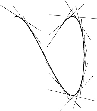
Similarly, instead of thinking of a curve—a conic, for example—as the path traced out by a moving point, we could think of it as traced by a moving line, as I have shown in Figure AG-4.

Can we construct our geometry around this idea? Yes, we can. This “line geometry” was actually worked out by the German mathematician Julius Plücker in 1829, which brings us back to the historical narrative.