This page intentionally left blank.

§6.1 THE BRITISH ISLES PRODUCED some fine mathematicians during the period from the late 16th century to the early 18th century, despite being busy with a civil war (1642–1651), a military dictatorship (1651–1660), a constitutional revolution (1688), and two changes of dynasty (Tudor to Stuart in 1603, and Stuart to Hanoverian in 1714).

I have already mentioned Thomas Harriot, whose sophisticated literal symbolism went largely unnoticed (except perhaps by Descartes). The Scotsman John Napier, though not significant as an algebraist, had discovered logarithms and presented them to the world in 1614. He also popularized the decimal point. William Oughtred, an English country parson, wrote on algebra and trigonometry and gave us the × sign for multiplication. John Wallis was the first to take up Descartes’ techniques and notations for analytical geometry (though he was a champion of Harriot, now long dead, and a vigorous proponent of the opinion that Descartes had gotten his notation from Harriot).

All these figures were, however, mere prologues to the arrival of Isaac Newton. This tremendous genius, by common agreement the greatest name in the history of science, was born on Christmas Day 1642,⁵⁵ to the widow of a prosperous farmer in Lincolnshire. The

subsequent course of his life and the character of the man have been much written about. Here are some words I myself wrote on those topics.

I cannot resist at this point telling my favorite Newton story, though I think it is quite well known. In 1696 the Swiss mathematician Johann Bernoulli posed two difficult problems to the mathematicians of Europe. Newton solved the problems the day he was shown them and passed on his solutions to the president of the Royal Society in London, who sent them to Bernoulli without telling him who had supplied them. As soon as he read the anonymous solutions, Bernoulli knew them to be Newton’s—“tanquam ex ungue leonem,” he said (“as by [his] claw [we know] the lion”).

That mighty claw scratched one great mark across the history of algebra.

§6.2 Newton⁵⁷ is famous for his contributions to science and for having invented calculus, but he is not well known as an algebraist. In fact, he had lectured on algebra at Cambridge University from 1673 to 1683 and deposited his lecture notes in the university library. Many years afterward, when he had left academic life and was established as master of the Royal Mint, his Cambridge successor, William Whiston, published the lectures as a book with the title Arithmetica universalis (Universal Arithmetic). Newton gave his permission for this publication, but only reluctantly, and he seemed never to have liked the book. He refused to have his name appear as author and even contemplated buying up the whole edition himself so that he could destroy it. Nor did Newton’s name appear on the English version (Universal Arithmetic), published in 1720, nor on the second Latin edition in 1722.⁵⁸

What most excites the interest of a historian of algebra, though, is not the Universal Arithmetic but some jottings a much younger Newton put down in 1665 or 1666 and that can be found in the first volume of his Collected Mathematical Works. They are in English, not Latin, and commence with the words:

These notes do not state any theorem. They suggest one, though; and the theorem is such a striking one that on the strength of the suggestion, mathematicians (as well as, in fact, the editor of the Collected Works) speak of Newton’s theorem.

Before presenting the theorem, I need to explain the concept of a symmetric polynomial. To keep things manageable, I’ll consider just three unknowns, calling them α, β, and γ. Here are some symmetric polynomials in these three unknowns:

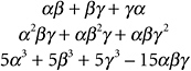
Here are some polynomials in α, β, and γ that are not symmetric:

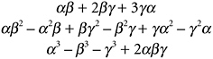
What distinguishes the first group from the second? Well, just by eyeball inspection, something like this: In the first group, everything that happens to α happens likewise to β and γ, everything that happens to β happens likewise to γ and α, and everything that happens to γ happens likewise to α and β. Things—addition, multiplication, combination—are happening to all three unknowns in a very even-handed way. This is not the case in the second group.

That is pretty much it, but the condition of being a symmetric polynomial can be described with more mathematical precision: If you permute α, β, and γ in any way at all, you end up with the same expression.

There are in fact five ways to permute α, β, and γ:

• Switch β and γ, leaving α alone.

• Switch γ and α, leaving β alone.

• Switch α and β, leaving γ alone.

• Replace α by β, β by γ, and γ by α.

• Replace α by γ, β by α, and γ by β.

(Note: A mathematician would try to persuade you that there are six permutations, the sixth being the “identity permutation,” where you don’t do anything at all. I shall adopt this point of view myself in the next chapter.)

If you were to do any of those things to any one of that first group of polynomials, you would end up with just the polynomial you started with, though perhaps in need of rewriting. If you do the last permutation to αβ + βγ + γα, for example, you get γα + αβ + βγ, which is the same thing, but written differently.

Another way of looking at this, and a useful (though not perfectly infallible!) way to check for symmetry when the polynomials are big and unwieldy, is to assign random numbers to α, β, and γ. Then the polynomial works out to a single numerical value. If this value is the same when you assign the same numbers to α, β, and γ in all possible different orders, it is symmetrical. If I assign the arbitrary numbers 0.55034, 0.81217, and 0.16110 to α, β, and γ in all six possible ways and work out the corresponding six values of αβ² − α²β + βγ² − β²γ + γα² − γ²α, I get 0.0663536 and −0.0663536 three times each. Not a symmetric polynomial: Permuting the unknowns gives two different values of the polynomial. (An interesting thing in itself—why two?—which I shall say more about later.)

All these ideas can be extended to any number of unknowns and to expressions of any level of complexity. Here is a symmetric polynomial of the 11th degree in two unknowns:

Here is a symmetric polynomial of the second degree in 11 unknowns:

Now, not all symmetric polynomials are equally important. There is a subclass called the elementary symmetric polynomials. For three unknowns the elementary symmetric polynomials are

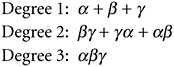
Of the examples I gave of symmetric polynomials above, the first is elementary, the other two are not.

You can think of the elementary symmetric polynomials in any number of unknowns as

If you are working with n unknowns, the list runs out after n lines because you can’t make an (n + 1)-tuplet out of n unknowns.

Now I can show you Newton’s theorem.

So although the other two examples of symmetric polynomials that I gave are not elementary, they can be written in terms of the three elementary symmetric polynomials I just showed. The second one is easy:

The third is a little trickier, but you can easily confirm that

By convention, and leaving it understood that we are dealing with some fixed number of unknowns (in this case three), the elementary symmetric polynomials are denoted by lowercase Greek sigmas, with a subscript to indicate degree. In this case, with three unknowns, the degree-1, degree-2, and degree-3 elementaries are called σ₁, σ₂, and σ₃. So I could write that last identity as

There is Newton’s theorem: Any symmetric polynomial in any number of unknowns can be written in terms of the sigmas, the elementary symmetric polynomials.

§6.3 What has all this got to do with solving equations? Why, just look back at those polynomials in α, β, γ, and so on, in §5.6, the ones Viète tinkered with. They are the elementary symmetric polynomials! For the general quintic equation x⁵ + px⁴ + qx³ + rx² + sx + t = 0, if the solutions are α, β, γ, δ, and ε, then σ₁ = −p, σ₂ = q, σ₃ = −r, σ₄ = s, and σ₅ = −t, where the sigmas are the elementary symmetric polynomials in five unknowns, which I actually wrote out in §5.6. A similar thing is true for the general equation of any degree in x.

Those jottings of Newton’s, the ones that lead us to Newton’s theorem, were, as I mentioned, done in 1665 or 1666, very early in Newton’s mathematical career. This was the time when, at age 21, just after he had obtained his bachelor’s degree, Newton had to go back to his mother’s house in the countryside because an outbreak of plague had forced the University of Cambridge to close. Two years later the university reopened, and Newton went back for his college fellowship and master’s degree. During those two years in the countryside, Newton had worked out all the fundamental ideas that underlay his discoveries in math and science. It is not quite the case, as folklore has it, that mathematicians never do any original work after age 30, but it is generally true that their style of thinking, and the topics that attract their keenest interest, can be found in their early writings.

Newton actually had a particular problem in mind when making those early jottings, the problem of determining when two cubic equations have a solution in common. However, this work on

1. symmetric polynomials in general, and

2. the relationships between the coefficients of an equation, and symmetric polynomials in the solutions of that equation

was crucial to further development of the theory of equations, and all that flowed from it, both within that theory and then beyond it into whole new regions of algebra. Symmetry … polynomials in the solutions as expressions in the coefficients … these were the keys to solving the great outstanding problem in the theory of polynomial equations at this point in the later 17th century, 120 years since the cracking of the cubic and the quartic: to find an algebraic solution for the general quintic.

§6.4 Speaking very generally, the 18th century was a slow time for algebra, at any rate by comparison with the 17th and 19th centuries. The discovery of calculus by Newton and Leibniz in the 1660s and 1670s opened up vast new mathematical territories for exploration, none of them algebraic in the sense I am using in this book. The area of math we now call “analysis”—the study of limits, infinite sequences and series, functions, derivatives, and integrals—was then new and sexy, and mathematicians took to it with enthusiasm.

There was a more general mathematical awakening, too. The modern literal symbolism developed for algebra by Viète and Descartes made all mathematical work easier by “relieving the imagination.” Furthermore, the growing acceptance of complex numbers stretched the imaginative boundaries of math. De Moivre’s theorem, which first appeared in finished form in 1722, may be taken as representative of early 18th-century pure mathematics. Stating that

the theorem threw a bridge between trigonometry and analysis and helped make complex numbers indispensable to the latter.

That is only to speak of pure mathematics. With the rise of science, the first stirrings of the Industrial Revolution, and the settling down of the modern European nation-system after the wars of religion, mathematicians were increasingly in demand by princes and generals. Euler designed the plumbing for Frederick the Great’s pal-

ace at Sans Souci; Fourier was a scientific adviser on Napoleon’s expedition to Egypt.

D’Alembert’s pioneering work on differential equations in the middle of the century was characteristic, and Laplace’s equation , which describes numerous physical systems where a quantity (density, temperature, electric potential) is distributed smoothly but unequally across an area or a volume, can be taken as representative of applied math at the century’s end.

Algebra was something of a bystander to all these glamorous developments. The general cubic and quartic equations had been cracked, but no one had much of a clue about how to proceed further in that direction. Viète, Newton, and one or two others among the most imaginative mathematicians had noticed the odd symmetries of the solutions of polynomial equations but had no idea how to make any mathematical profit from these observations.

There was, however, one other problem that mathematicians struggled with all through the 18th century and that I ought to cover here. This was the problem of finding a proof for the so-called fundamental theorem of algebra, hereinafter the FTA. I write “so-called” because the theorem always is so called, yet its status as implied by that name is considerably disputed. There are even mathematicians who will tell you, in the spirit of Voltaire’s well-known quip about the Holy Roman Empire, that the FTA is neither fundamental, nor a theorem, nor properly within the scope of algebra. I hope to clarify all that in just a moment.

The FTA can be stated very simply, if a little roughly, in the context of polynomial equations, as: Every equation has a solution. To be more precise:

Ordinary real numbers are to be understood here as just particular cases of complex numbers, the real number a as the complex number a + 0i. So equations with real-number coefficients, like all the ones I have displayed so far, come under the scope of the FTA. Every such equation has a solution, though the solution may be a complex number, as in the case x² + 1 = 0, satisfied by the complex number i (and also by the complex number −i).

The FTA was first stated by Descartes in La géométrie (1637), though in a tentative form, as he was not at ease with complex numbers. All the great 18th-century mathematicians had a go at trying to prove it. Leibniz actually thought he had disproved it in 1702, but there was an error in his reasoning, pointed out by Euler 40 years later. The mighty Gauss made it the subject of his doctoral dissertation in 1799. Not until 1816 was a completely watertight proof given, though—also by Gauss.

To clarify the mathematical status of the FTA, you really need to study a proof. The proof is not difficult, once you have made friends with the complex plane (see Figure NP-4) and can be found in any good textbook of higher algebra.⁵⁹ What follows is the merest outline.

§6.5 Proof of the Fundamental Theorem of Algebra

It is the case with complex numbers, as with real numbers, that higher powers easily swamp lower ones, a thing I mentioned in §CQ.3. Cubes get seriously big much faster than squares, and fourth

powers much faster than cubes, and so on. (Note: The word “big,” when applied to complex numbers, means “far from the origin,” or equivalently “having a large modulus.”) For big values of x, therefore, the polynomial in that box above looks pretty much like xⁿ with some small adjustments caused by the other terms.

If x is zero, on the other hand, every term in the polynomial is equal to zero, except for the last, “constant,” term. So for tiny values of x, the polynomial just looks like that last constant term. (The constant term in x² + 7x − 12, for instance, would be −12.)

If you change x smoothly and evenly, then x², x³, x⁴, and all higher powers will also change smoothly and evenly, though at different speeds. They will not suddenly “jump” from one value to another.

Given those three facts, consider all the complex numbers x with some given large modulus M. These numbers, if you mark them in the complex plane, form the circumference of a perfect circle of radius M. The corresponding values of the polynomial form, but only approximately, the circumference of a much bigger circle, one with radius Mⁿ. (If a complex number has modulus M, its square has modulus M² and so on. This is easy to prove.) That’s because xⁿ has swamped all the lower terms of the polynomial.

Gradually, smoothly, shrink M down to zero. Our perfect circle—all the complex numbers with modulus M—shrinks down to the origin. The corresponding values of the polynomial shrink down correspondingly, like a loop of rope tightening, from a vast near-circle centered on the origin to the single complex number that is the constant term in the polynomial. And in shrinking down like this, the tightening polynomial loop must at some point cross the origin. How else could all its points end up at that one complex number?

Which proves the theorem! The points of that dwindling loop are values of the polynomial, for some complex numbers x. If the loop crosses the origin, then the polynomial is zero, for some value of x. Q.E.D. (Though you might want to give a moment’s thought to the case where the constant term in the polynomial is zero.)

§6.6 The unhappy thing—from an algebraic point of view, I mean—about this proof is that it depends on the matter of continuity. I argued that as x changes gradually and slowly, so does the corresponding value of the polynomial. This is perfectly true, but it is only true because of the nature of the complex number system, in which you can glide without any jumps or bumps from one number to another, over the dense infinity of numbers in between.

Not all number systems are so accommodating. Number systems are many and various in modern algebra, and we can set up polynomials, and polynomial equations, in all of them. Not many are as friendly as the system of complex numbers, and the FTA is not true in all of them.

From the point of view of modern algebra, therefore, the FTA is a statement about a property of the complex number system, the property known in modern jargon as algebraic closure. The system of complex numbers (it says) is algebraically closed—which is to say, any single-unknown polynomial equation with coefficients in the system has a solution in the system. The FTA is not a statement about polynomials, equations, or number systems in general. That is why some mathematicians will take haughty pleasure in telling you that it is not fundamental; and while it is probably a theorem, it is not really a theorem in algebra but in analysis, where the notion of continuity most properly belongs.⁶⁰