Human Factors Guidelines for Road Systems: Third Edition (2025)
Chapter: 27 Tutorials

CHAPTER 27
Tutorials
Tutorial 1: Real-World Driver Behavior Versus Design Models
Tutorial 2: Diagnosing Sight Distance Problems and Other Design Deficiencies
Tutorial 3: Detailed Task Analysis of Curve Driving
Tutorial 4: Determining Appropriate Clearance Intervals
Tutorial 5: Determining Appropriate Sign Placement and Letter Height Requirements
Tutorial 6: Calculating Appropriate CMS Message Length under Varying Conditions
Tutorial 7: Joint Use of the Highway Safety Manual and the Human Factors Guidelines for Road Systems
Tutorial 1: Real-World Driver Behavior Versus Design Models
Much of the information on sight distance presented in Chapter 5 reflects the application of empirically derived models to determine sight distance requirements. Such models, while valuable for estimating driver behavior across a broad range of drivers, conditions, and situations, have limitations.
This tutorial discusses how driver behavior, as represented in sight distance models, may differ from actual driver behavior. The design models presented in Chapter 5 use simplified concepts of how the driver thinks and acts. This simplification should not be viewed as a flaw or error in the sight distance equations. These models are very effective methods for bringing human factors data into design equations in a manner that makes them accessible and usable. After all, the intent of a sight distance equation is not to reflect the complexities of human behavior but to bring what we know about it into highway design in a concise, practical way. However, like any behavioral model, models for deriving sight distance requirements are not precise predictors of every case, and there may be some limitations to their generality. Therefore, certain basic principles of human behavior in driving situations can help better interpret these models and understand how they may differ from the range of real-world driving situations.
Sight distance formulas for various maneuvers (presented in Chapter 5) differ from one another, but they share a common simple behavioral model. The model assumes that some time is required for drivers to perceive and react to a situation or condition requiring a particular driving maneuver (i.e., the perception-reaction time, PRT), which is followed by the maneuver time (MT) and distance to execute the maneuver. Sight distance equations for some maneuvers may contain additional elements or assumptions; however, all have this basic two-stage model at their core.
The two equations that follow show two versions of the general, two-component model. In both versions, the first term shows the distance traveled during the PRT component, and the second term shows the distance traveled during the MT component. The difference is that the first equation shows a case where the distance traveled while executing the maneuver is based on the time required to make that maneuver (for example, the time to cross an intersection from a Stop), while the second equation shows a case where the distance traveled while executing the maneuver is based directly on the distance required to complete the maneuver (for example, braking distance for an emergency stop). For both forms of this general equation, vehicle speed (V) influences the second (MT) component.
The general form of the sight distance equation is:

Long Description.
d subscript SD equals k V t subscript prt plus k V t subscript man

Long Description.
d subscript SD equals V t subscript prt plus V d subscript man superscript v
Where:
dSD = required sight distance
V = velocity of the vehicle(s)
tprt = perception-reaction time
tman = maneuver time
dmanv = Distance required to execute a maneuver at velocity V
k = A constant to convert the solution to the desired units (feet, meters)
This model shows that the sight distance requirement is composed of (at least) two distances: a distance traveled while the driver perceives and evaluates a situation (determined by PRT and vehicle speed) and a distance traveled while executing the maneuver (determined by maneuver time/distance and vehicle speed). Figure 27-1 depicts the activities and sequence of activities associated with this simple model. As the figure shows, the PRT component is itself viewed as a series of steps. These individual steps are not explicit in the design equation but are included in the assumptions that underlie the PRT value. Design equations and their assumptions for specific maneuvers were discussed in Chapter 5. The sequential model of driver behavior shown in Figure 27-1 is a shared common conceptual underpinning of various sight distance equations.
However, in some respects, we can consider this model to be a “convenient fiction,” in part because it depicts a simple, fixed, linear, and mechanistic process. While the model provides a useful basis for deriving approximate quantitative values for design requirements that work for many situations, real-world driving behavior is far more complex than the model suggests. While highway designers and traffic engineers are often required to work with less complex (i.e., imperfect) models of human visual perception, attention, information processing, and motivation, it is important that they understand the factors that may affect the application of design sight distance models in specific situations. Such an understanding will help them prevent, recognize, or deal with sight distance issues that may arise. For a particular situation, the standard sight distance design equation might either underestimate or overestimate the actual needs of a driver. Subsequent sections of this tutorial deal with specific factors that affect the driver response and provide guidance for working with them. Before considering these specific factors, it will be useful to have an appreciation for how the simple driver models that underlie sight distance requirements contrast with the real complexities of driver behavior.
There are a number of factors or conditions associated with driver responses to a hazardous event or object that are not reflected in the basic sight distance model, but nonetheless can have a profound effect on driver behavior and overall roadway safety:
- Conditions or events that occur prior to a hazardous event/object becoming visible to the driver
- How and when the driver processes relevant information
- Driving as an “episodic” activity versus driving as a “smooth and continuous” activity
- The nature of the hazardous object or event
- The nature of the driverʼs response
- Individual differences across drivers
- The quality and applicability of the empirical research used to develop the driver models
Each of these is discussed in more detail in the sections that follow.
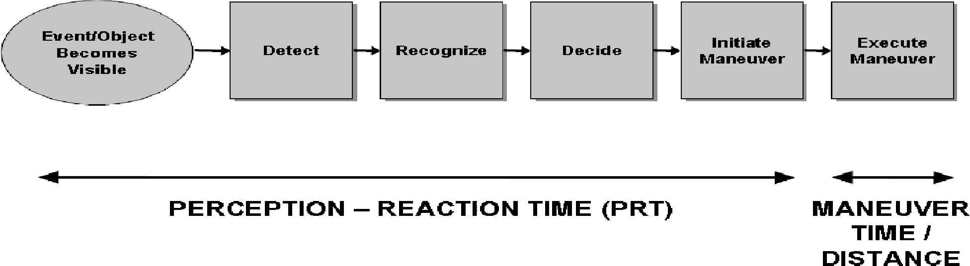
Long Description.
The first element of the flowchart is an oval-shaped element that says Event/Object Becomes Visible. There are then five square elements that say Detect; Recognize; Decide; Initiate Maneuver; and Execute Maneuver. Below the flowchart are two line segments labeled Perception-Reaction Time (PRT) and Maneuver Time / Distance. The PRT segment covers the oval element and the first four square elements and the Maneuver Time / Distance segment covers the Execute Maneuver element.
Conditions or Events that Occur Prior to a Hazardous Event/Object Becoming Visible to the Driver
The model shown in Figure 27-1 is not sensitive to events that happen prior to the moment that the hazardous object or event becomes visible to the driver. In reality, the driverʼs ability to react to a hazardous object or event may be strongly influenced by previously occurring conditions or events. For example, drivers traveling on a roadway with few access points and little traffic may be unprepared to stop for a slow-moving vehicle ahead. In contrast, if drivers had been encountering numerous commercial driveways and intersections with entering truck traffic, they might more readily react. Roadway design and operational features in advance of a hazardous event/object becoming visible are potentially important influences on behavior that are not explicit in the basic sight distance model. Figure 27-2 shows an expansion of the basic model, with added “driver state” factors (e.g., anticipation, situational awareness, caution, and locus of attention) that increase or decrease the driverʼs cognition preparation for a hazardous condition or event.
In Figure 27-2, an additional component to the model is shown prior to the event becoming visible. One element of the additional component is cognitive preparation. This general term encompasses the various active mental activities that can influence response times and decisions, such as driver expectancies, situational awareness, a general sense of caution, and where attention is being directed by the driver. Part II: Bringing Road User Capabilities into Highway Design and Traffic Engineering Practice provides some further explanation of these factors. As the arrows in the figure show, the driverʼs cognitive preparation as he or she encounters a hazardous object or event can influence the speed of detection, the speed and accuracy of recognizing the situation, and the speed and type of decision made about how to respond. The critical point is that the PRT associated with a particular hazardous object or event is influenced by the conditions or events preceding the driverʼs perception of the hazardous object or event.
The second element in the additional component in Figure 27-2 that occurs prior to the driverʼs perception of the hazardous object or event is speed selection. As discussed earlier, speed can have perceptual effects, influencing how easily a target object is detected or how accurately gaps are judged. Speed may affect the driverʼs sense of urgency, which can influence what maneuver options are considered and their relative appeal. Speed also may directly affect the difficulty, as well as the required time or distance, of the maneuver. Therefore, the driverʼs speed choice prior to the event may influence the driverʼs decision process; it may also influence the time available for the driverʼs response.
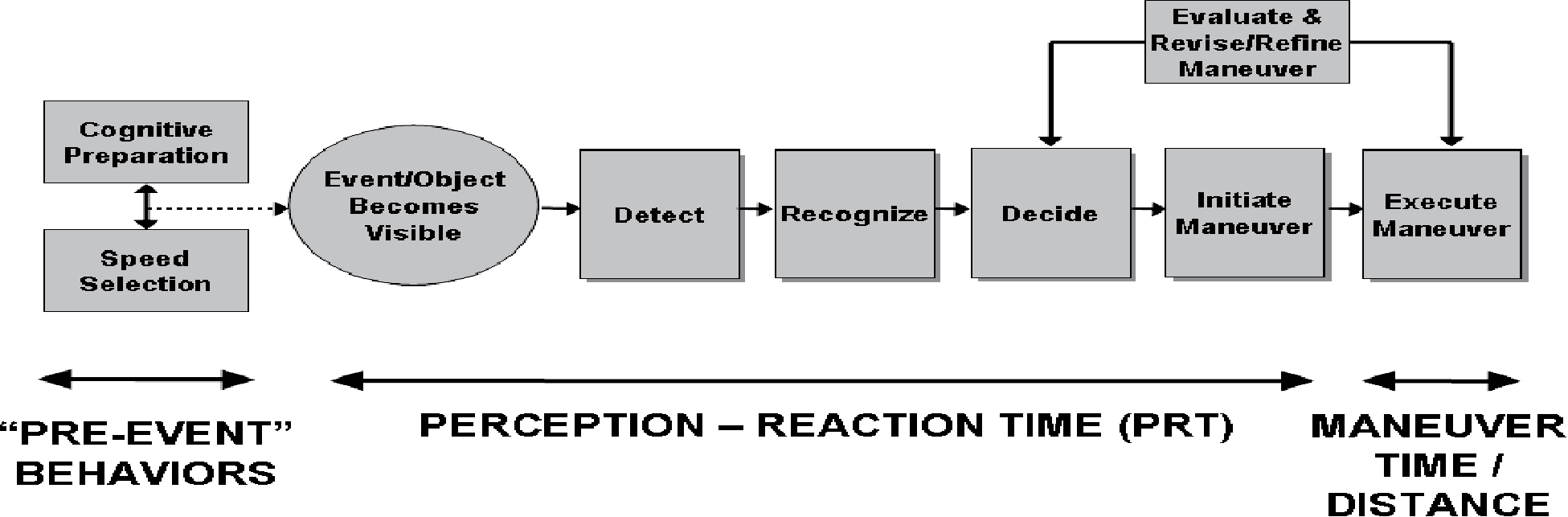
Long Description.
The major components of the model are “pre-event” behaviors, perception-reaction time (PRT), and maneuver time and distance. In the Pre-event behaviors segment, two boxes are connected by a vertical double-headed arrow. The first box says Cognitive Preparation and the second box says Speed Selection. At the middle of the double-headed arrow connecting the first two boxes a dotted arrow leads to an oval that says Event/Object Becomes Visible. There are then five square elements connected by arrows that say Detect; Recognize; Decide; Initiate Maneuver; and Execute Maneuver. A line segment below the oval and the first four boxes says Perception – Reaction Time (PRT). A line segment below the Execute Maneuver box says Maneuver Time / Distance. Above these boxes is a box that says Evaluate and Revise / Refine Maneuver, which is connected to the Decide and Execute Maneuver boxes by single-headed arrows.
The basic sight distance behavioral model (Figure 27-1) makes assumptions about driver cognitive state and speed choice as the hazardous event is encountered. In reality, the driver does not arrive at the situation as a “blank slate.” The locus of a sight distance problem, or its solution, therefore may turn out to be in advance of the problem site itself.
How and When the Driver Processes Relevant Information
The basic sight distance model shows a chain of mental and physical events taking place in the following sequential fashion:
- A hazardous object or event becomes visible.
- The presence of this object or event is detected by the driver.
- The object or event is recognized and understood by the driver.
- The driver makes a decision about what maneuver is needed to avoid or respond to the object or event.
- The maneuver is initiated.
- Once initiated, the maneuver is fully executed.
Each event in this chain takes some amount of time to occur, and—according to the basic model—one step does not begin until the previous step is complete. This assumed “serial processing” model is indeed one way a driver might respond, but it may not be typical. For example, if a driver sees some vague object ahead of the vehicle that might or might not be in the roadway, he or she may begin to brake even before the object is fully recognized. Also, once the object is fully recognized, the maneuver may be reconsidered (e.g., stopped, slowed, accelerated, or otherwise revised). Contrary to the serial processing assumed by the basic model, the mental processes shown by the various boxes in Figure 27-1 may actually occur in parallel, in a different sequence, or with modifications (feedback loops) as the process progresses. The assumed linear response sequence is therefore a simplified case used for design purposes. It should not be viewed as a universal or invariant representation of the more complex perceptual and cognitive activity in complex driving situations.
Importantly, consistency in geometric design is required to meet driver expectations and to avoid surprising the driver.
Driving as an “Episodic” Activity versus Driving as a “Smooth and Continuous” Activity
Related to the previous point, the basic sight distance model reflects an “episodic” perspective of real-world driving. That is, some object or event becomes visible, and some driver maneuver(s) in response to the object or event are initiated and executed. Then, another object or event becomes visible, and another maneuver takes place. Real-world driving however, is normally smooth and continuous; it is not a jerky sequence of separate, individual episodes. Yet for ease of analysis, we often break driver behavior into individual events each requiring their own separate response, or we treat the roadway as a succession of discrete segments or zones. To the driver, though, the roadway and the driving task are generally smooth and continuous. Real drivers do not just react to events that randomly occur; they plan and predict and manage and adapt to events as they go along. Adopting an “episodic” perspective is useful for developing models of driver behavior that are both simple and reasonably predictive. A “smooth and continuous” perspective of real-world driving is much more difficult to model and quantify, especially in a manner that will easily generate a simple design parameter. From a human factors perspective, sight distance models are based on a little bit of driver performance data that describe how a driver might react, but may not reflect how drivers always or even typically behave. The use and
application of the simpler sight distance model is generally reasonable from a design perspective, however, because it is somewhat conservative. Specifically, those drivers who encounter a situation without planning or anticipation are those most likely to be in need of the full sight distance requirement.
The Nature of the Hazardous Object or Event
For each sight distance design application, the analysis is based around some object, event, or roadway feature to which the driver must respond with a driving maneuver. That object, event, or roadway feature might be debris in the roadway, braking by a vehicle ahead, an approaching vehicle on a conflicting path, a freeway lane drop, a change in signal phase, a pedestrian entering the road, a railroad gate, an animal, a vehicle entering from a driveway, or many other things. The PRT process begins with the potentially hazardous object or event (the “visual target”) becoming visible to the driver, followed by some time to visually detect and recognize that target. Design equations must include some estimate of when a target becomes visible and how long it will take drivers to react. The many examples of potential hazards suggest the range of variation in visual targets; therefore, any single estimate for either when the targets will become visible or how long it will take drivers to react to them will be based on simplified assumptions. A target object may be large or small, bright or dull, familiar or unfamiliar, moving or stationary, or have other attributes that affect the driverʼs ability to accurately and quickly detect and recognize it. Explicitly or implicitly, design equations must make some assumption about the characteristics of the visual target. Furthermore, visibility conditions may vary with weather, glare, light condition, roadway lighting, and intervening traffic (especially truck traffic). Again, design equations must be based on some assumption about visibility conditions.
A PRT model requires the user to be able to specify the point in time or space that the hazard becomes visible to the driver. However, this too may be an oversimplification. For example, there is usually no sharp threshold where an object in the road suddenly goes from being invisible to visible. Most hazards do not occur all at once, but evolve over some time, such as a vehicle moving into a lane in front of a driver. Some events might have a preview, such as a vehicle positioned in a driveway prior to its pulling out or children playing near the road prior to entering the road. Some events might have multiple cues; for example, a freeway lane drop has an initial taper, lane markings, and the point where the lane finally disappears. Sometimes the important visual target is not the hazard object or event itself but a cue about the hazard; for example, brake lights on a vehicle ahead may be a warning cue about a sudden severe deceleration, but they may also reflect a minor tap on the brake. Drivers cannot respond to the brake light in the same way they respond to recognition of the actual deceleration.
To summarize, the driverʼs response to a hazardous event or object will reflect specific physical characteristics, visibility conditions, and the evolving nature of the hazard itself.
The Nature of the Driverʼs Response
The behavioral components of sight distance models are based around some very specific maneuver in response to the object/event, with fixed assumptions about response parameters. For example, when responding to an unexpected need to stop, AASHTO (2004) assumes a braking maneuver with a deceleration of 3.4 m/s2 (11.2 ft/s2). Braking may be a reasonable response to assume, and 3.4 m/s2 may be a reasonable deceleration to assume, but this certainly does not mean that braking at this level is always the driverʼs response to an unexpected hazard. The maneuver time and maneuver distance components of sight distance models are in many cases based on good empirical research and human factors considerations and work well for most applications. Still, the use of a single standard value is a convenient simplification. Actual
maneuvers can be influenced by various factors. The perceived urgency of the situation (based on available time/distance, driver/vehicle capabilities) determines options and shapes the way drivers respond, and often multiple options are available to the driver. For example, for an unanticipated stop, a driver may brake severely, or brake gradually and steer around, or swerve sharply. The surrounding physical, traffic, and social environment will affect these options: is there a lane or shoulder to steer around, are there adjacent or following vehicles, is the obstacle a piece of debris or a child, is there a passenger in the vehicle? Drivers also make trade-offs between speed versus control when executing maneuvers. The AASHTO deceleration value of 3.4 m/s2 represents an estimate of a “comfortable deceleration” with which almost all drivers can maintain good vehicle control. In this sense, it is appropriate for general design but does not necessarily describe what drivers can do or actually do under all conditions or circumstances. Furthermore, once a driver initially selects and begins to execute a particular maneuver, the maneuver is not simply executed in a fixed manner. As Figure 27-2 illustrates, the situation is monitored and the maneuver is re-evaluated as it is being executed. The response may be refined or modified as it progresses. Drivers may not respond to a situation with a maximum response (e.g., maximum braking or steering), but may initiate a more controlled action and monitor the situation before committing to a more extreme action. For instance, they may begin gradual braking and check their mirrors for following traffic before decelerating more sharply or swerving.
Individual Differences Across Drivers
The diverse driving population ranges widely in capabilities and behaviors. Drivers vary in experience, visual acuity, contrast sensitivity, useful field of view, eye height, information processing rate, tolerance for deceleration, physical strength, and other factors related to PRT and MT. A design equation will typically be based around a design driver with some assumed set of attributes. To be conservative, the assumptions do not usually represent a typical driver, but rather reflect less capable drivers (e.g., 15th percentile in terms of some attribute). Assumptions are made about the state of the driver as well. For example, data are generally based on drivers who are sober and alert. Yet impaired or fatigued drivers may represent a large part of the crash risk. Alcohol, drugs, medication, and fatigue can have dramatic effects on the psychological processes that underlie PRT and MT. Driver distraction by activity within the vehicle is also a common occurrence that is not reflected in the design model. In-vehicle technologies, such as cell phones, navigation systems, and infotainment systems, are increasingly common. The multitasking driver is an increasing concern, but PRT models do not reflect these issues.
The Quality and Applicability of the Empirical Research Used to Develop the Driver Models
The values used in design equations may or may not be derived from good empirical sources. In some cases (e.g., brake reaction time), there are numerous empirical studies and reasonably good agreement among them. In other cases, empirical data are very limited, are of lesser quality, or are only weakly applicable to the design issue in question. The quality and applicability of the numbers that come from empirical studies are sometimes questionable on a number of grounds: the sample of drivers may be small or unrepresentative; the situations evaluated may be limited and may not generalize well; the research may be out of date (given changes in roadways, traffic, vehicles, traffic control devices, and driver norms); the research setting (test track, simulator, laboratory) may lack validity; and results may conflict with results from other studies. It would be wrong to assume that sight distance design equations are necessarily based on a strong, high-quality empirical foundation that readily generalizes to all cases.
Another concern related to data quality and applicability is the inability of general design equations based on simple behavioral models to incorporate site-specific considerations. Empirical
observations made at the site may be at variance with the behaviors predicted under a general model. Even when design equations are based on “good” data, the generality of the models suggests that it may be prudent to adjust models in accordance with empirical data collected at a specific site.
In summary, sight distance requirements are based on a highly simplified and mechanistic model of driver behavior and capabilities. This approach is reasonable and generally successful. The general assumptions often work well enough to approximate the needs of most drivers; however, it is important to recognize that this simple model has a number of limitations as a description of actual driver performance. When diagnosing or addressing difficult sight distance problems, it may be useful for the highway designer or traffic engineer to recognize how design models simplify driver actions and to acknowledge the more complex realities of driver perception and behavior.
Tutorial 2: Diagnosing Sight Distance Problems and Other Design Deficiencies
Introduction
The previous sections of this document—especially Chapter 5—have provided design guidelines for human factors aspects of various sight distance concepts. However, for users to implement these guidelines in a practical sense, it is desirable to provide a procedure for their operational application. Therefore, this section comprises a hands-on tool practitioners can use to apply human factors techniques to analyze sight distance problems and other design deficiencies at a selected highway location.
A starting point for the development of the current procedure was a review of previously documented procedures for conducting on-site driving task analyses (Alexander and Lunenfeld, 2001), which applied techniques such as commentary drive-through procedures to generate subjective-scaled ratings of hazard severity and information load. The current in situ sight distance diagnostic procedure includes the application of previously available engineering tools, e.g., AASHTO (2011a) analyses of geometric requirements and Manual on Uniform Traffic Control Devices (MUTCD) traffic control device requirements (FHWA, 2023b), and augments these techniques with those sight distance concepts presented in Chapter 5 of this HFG.
This sight distance diagnostic procedure consists of a systematic on-site investigation technique to evaluate the highway environment in relation to the concepts of interest, including stopping sight distance (SSD), passing sight distance (PSD), intersection sight distance (ISD), or decision sight distance (DSD). The highway location is surveyed, diagrammed, and divided into component sections based on specific driving demands (e.g., the requirement to perform a maneuver). Then, each section is analyzed in terms of its suitability to support the required task (e.g., the information provided to the driver and allotted time to complete the required task). This procedure enables the practitioner to compare the available sight distance with the required sight distance to safely perform the driving task.
The Six-Step Procedure
The procedure consists of the following six steps:
- Collect field data to describe roadway characteristics and other environmental factors affecting sight distance requirements and driver perception of a potential hazard.
- Conduct engineering analyses using traditional techniques, such as AASHTO design criteria and MUTCD compliance, to initially assess site characteristics and deficiencies.
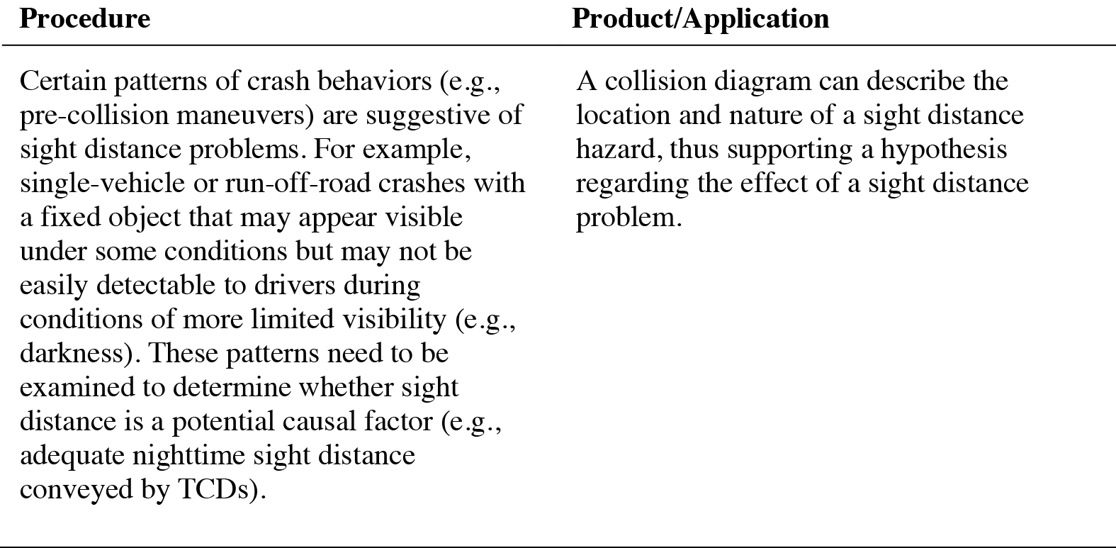
- Examine crash data and prepare a collision diagram to seek possible associations between safety and a sight distance problem.
- Establish component roadway segments in which drivers respond to specific visual cues to initiate a maneuver to avoid a hazard.
- Analyze driving task requirements (PRT and MT) and determine the adequacy of each component roadway section to support these requirements.
- Develop engineering strategies for the improvement of sight distance deficiencies.
A flow diagram overview of the process is shown in Figure 27-3. Following the description of the six-step procedure, an example application is provided.
Step 1: Collect Field Data
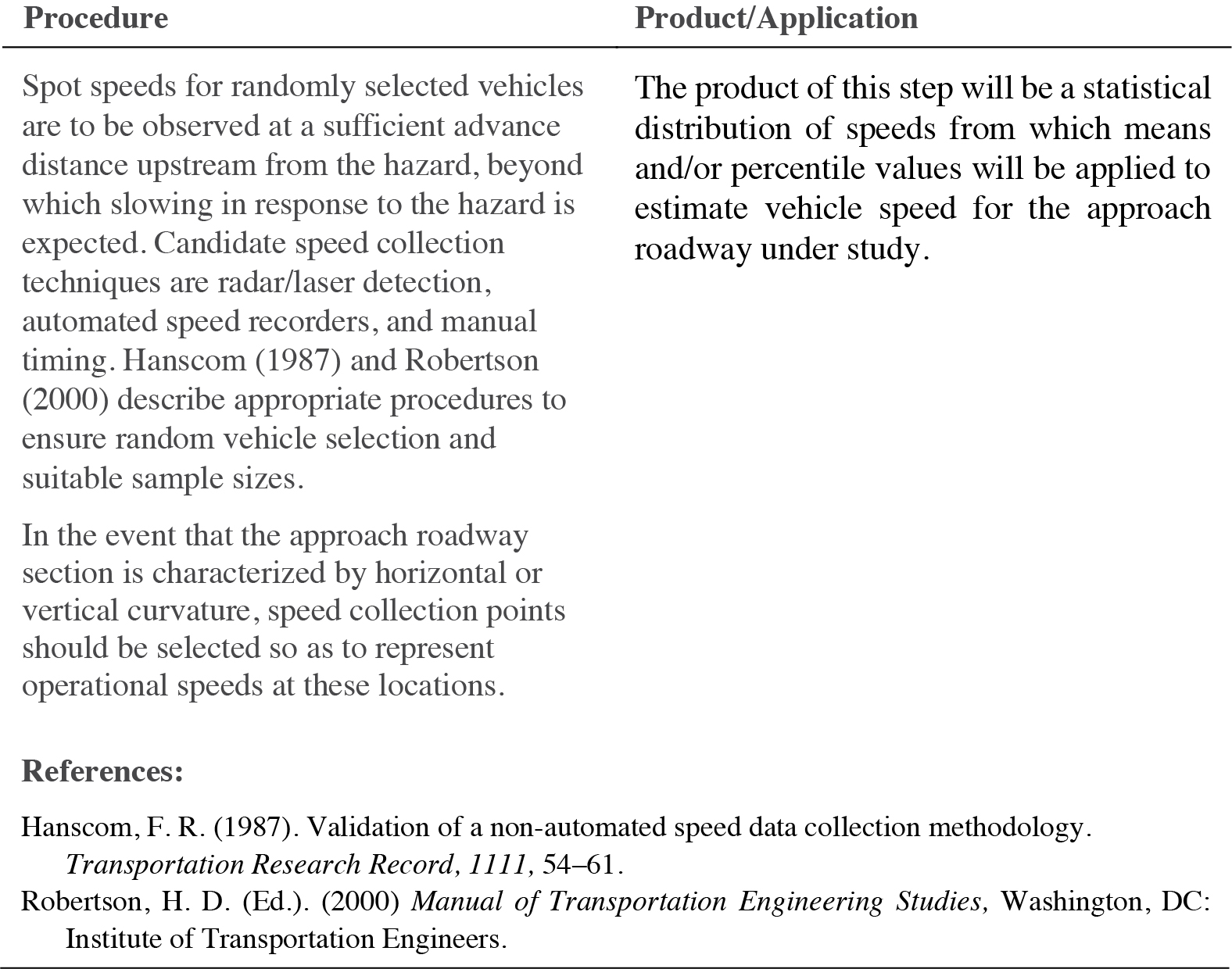
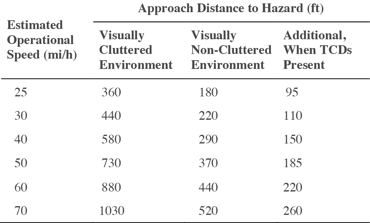
This step involves making specific field measurements and observations. Data are to be gathered both at the location of the designated hazard as well as the approach roadway section immediately in advance of the hazard. Approach distances over which field measurements should be gathered are determined from Table 27-1 at the end of this step. Approach distances were derived from approximated perception-reaction and sign reading times applied to the designated operating speeds.
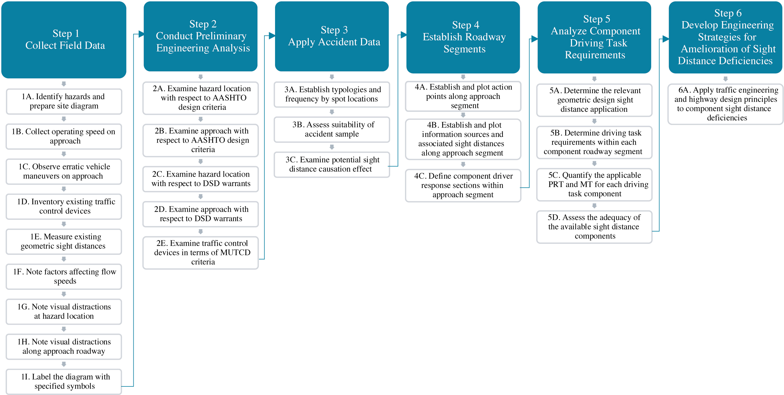
Long Description.
The following steps are depicted in the flow chart: Step 1 Collect Field Data 1A. Identify hazards and prepare site diagram 1B. Collect operating speed on approach 1C. Observe erratic vehicle maneuvers on approach 1D. Inventory existing traffic control devices 1E. Measure existing geometric sight distances 1F. Note factors affecting flow speeds 1G. Note visual distractions at hazard location 1H. Note visual distractions along approach roadway 1I. Label the diagram with specified symbols Step 2 Conduct Preliminary Engineering Analysis 2A. Examine hazard location with respect to AASHTO design criteria 2B. Examine approach with respect to AASHTO design criteria 2C. Examine hazard location with respect to DSD warrants 2D. Examine approach with respect to DSD warrants 2E. Examine traffic control devices in terms of MUTCD criteria Step 3 Apply Accident Data 3A. Establish typologies and frequency by spot locations 3B. Assess suitability of accident sample 3C. Examine potential sight distance causation effect Step 4 Establish Roadway Segments 4A. Establish and plot action points along approach segment 4B. Establish and plot information sources and associated sight distances along approach segment 4C. Define component driver response sections within approach segment Step 5 Analyze Component Driving Task Requirements 5A. Determine the relevant geometric design sight distance application 5B. Determine driving task requirements within each component roadway segment 5C. Quantify the applicable PRT and MT for each driving task component 5D. Assess the adequacy of the available sight distance components. Step 6 Develop Engineering Strategies for Amelioration of Sight Distance Deficiencies. 6A. Apply traffic engineering and highway design principles to component sight distance deficiencies
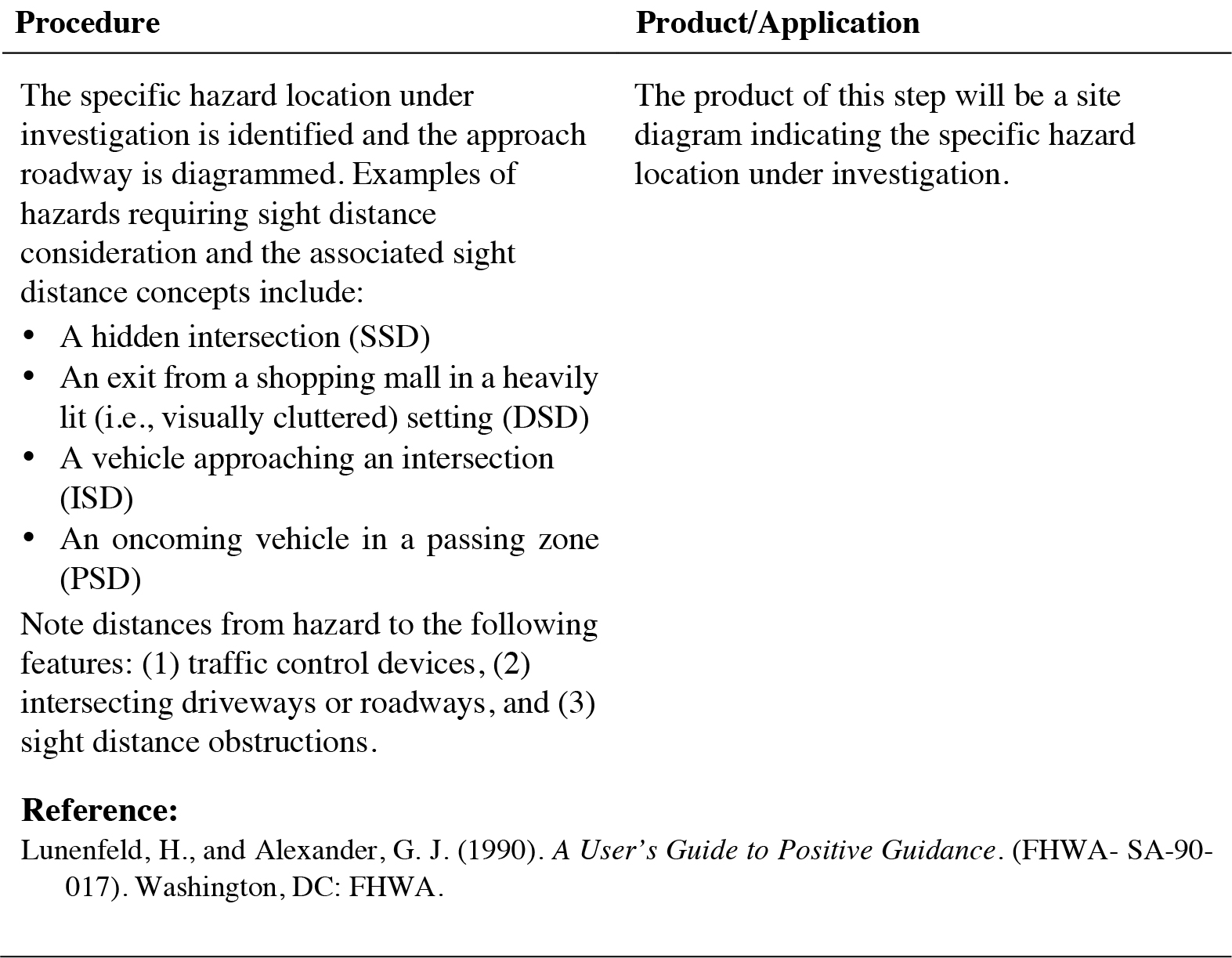
Step 1A: Identify Hazard and Prepare Site Diagram
Step 1B: Collect Operating Speed on Approach
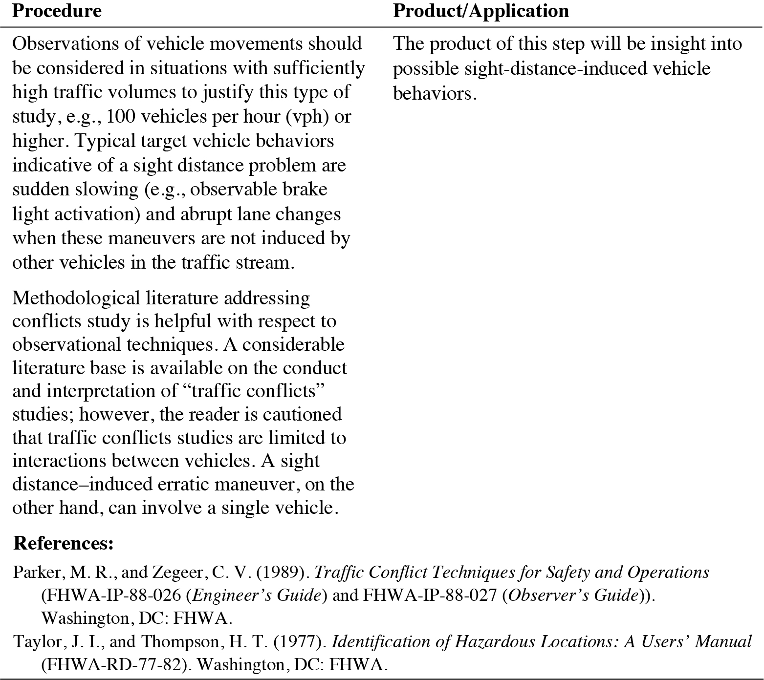
Step 1C: Observe Erratic Vehicle Maneuvers on Approach
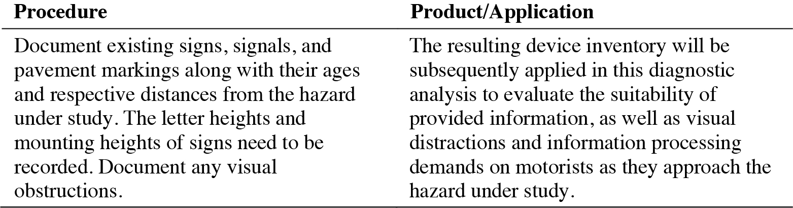
Step 1D: Inventory Existing Traffic Control Devices
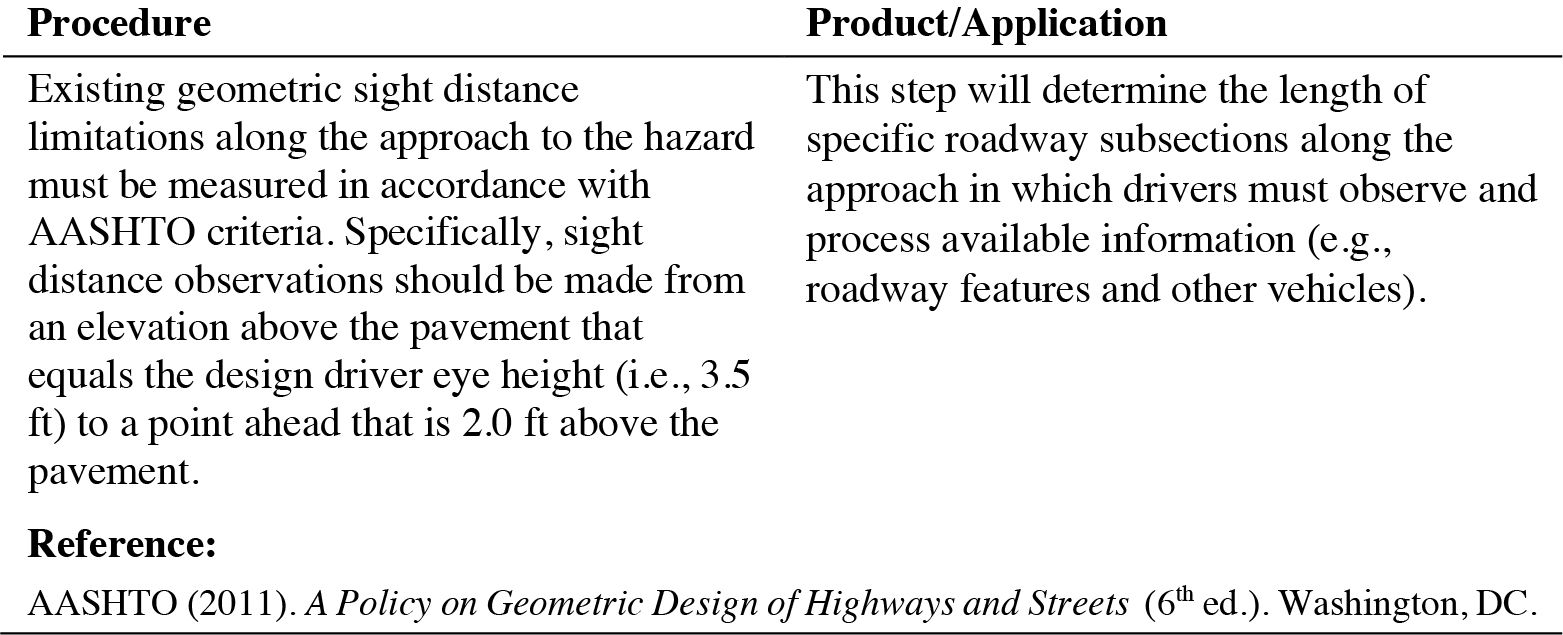
Step 1E: Measure Existing Geometric Sight Distances
Step 1F: Note Factors Affecting Flow Speeds
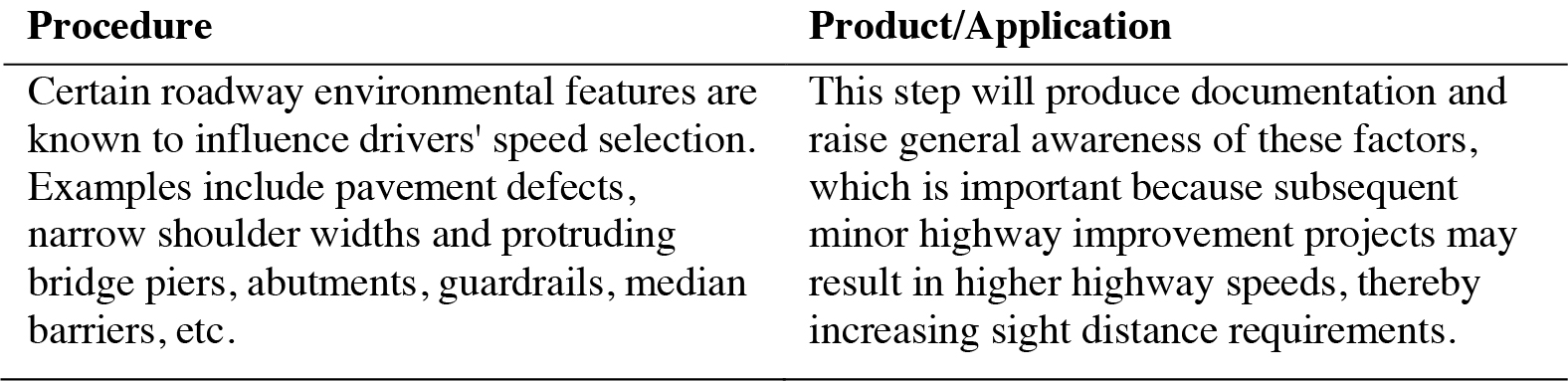
Step 1G: Note Visual Distractions at Hazard Location
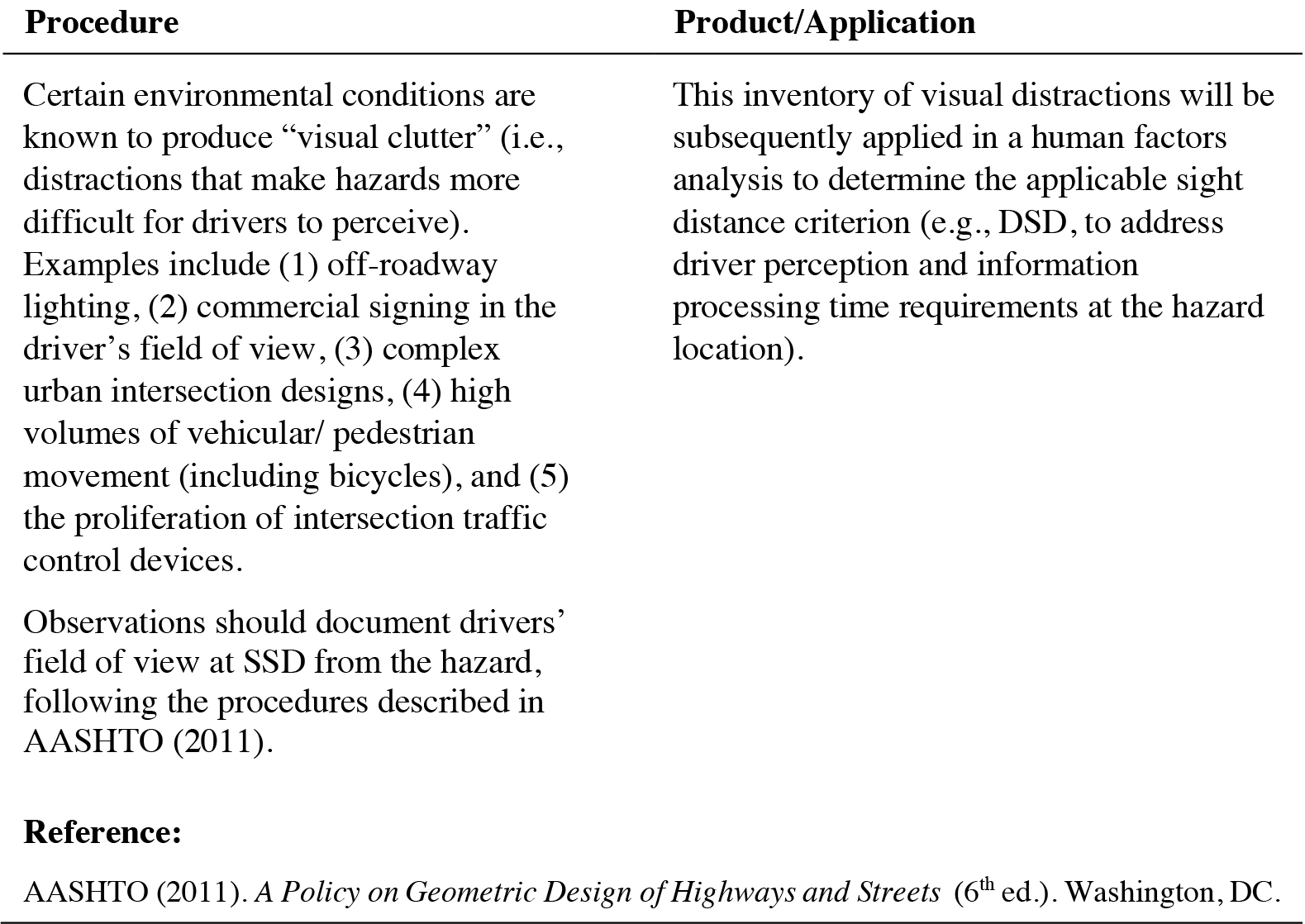
Step 1H: Note Visual Distractions Along Approach Roadway
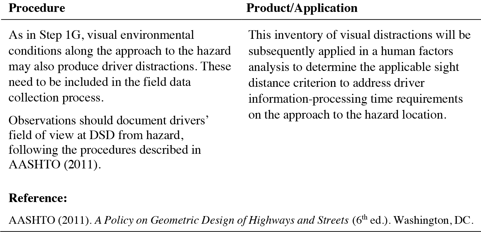
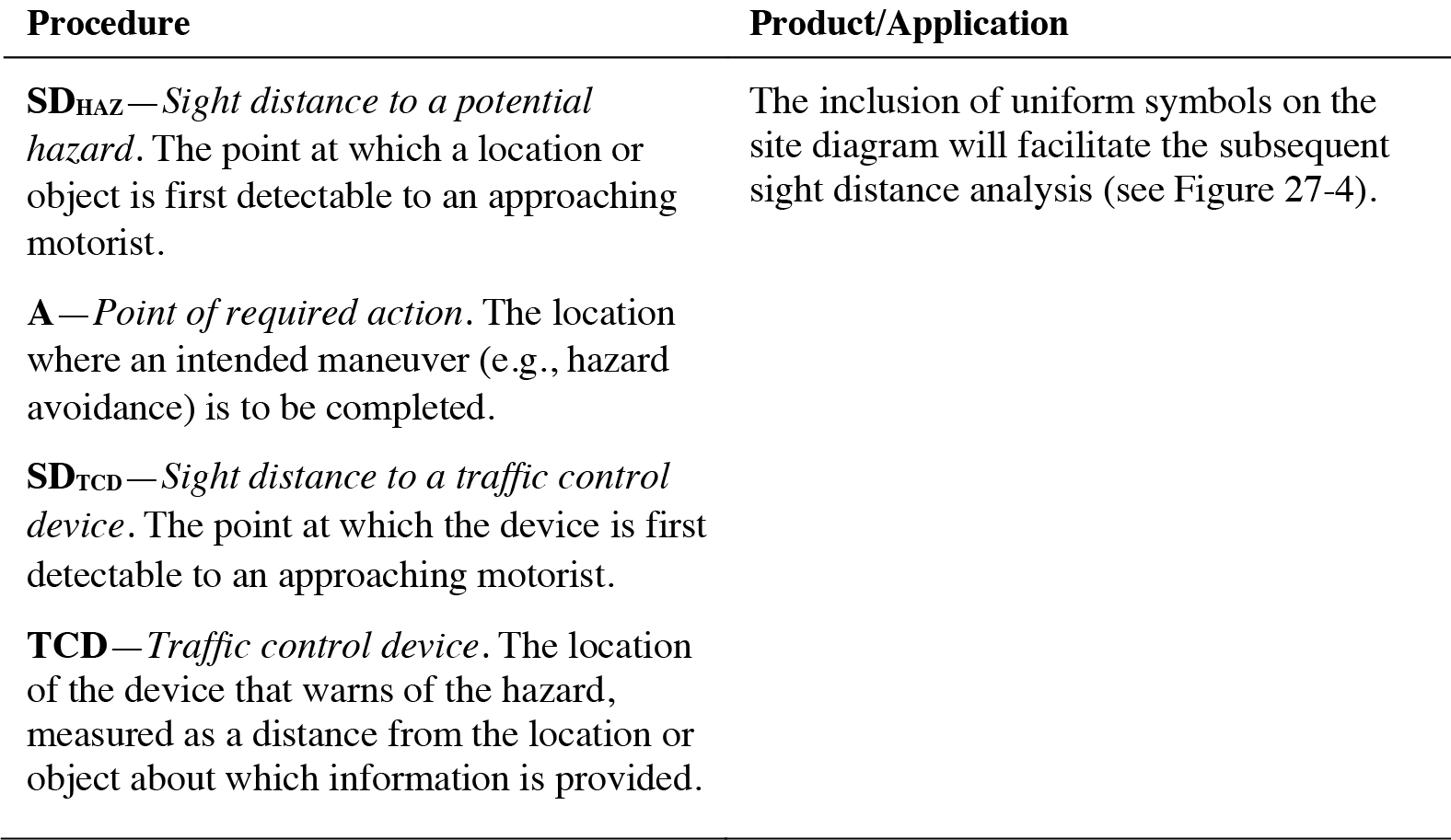
Step 1I: Label the Diagram with Specified Symbols
Long Description.
Column heading 1 is Estimated Operational Speed in miles per hour. Column headings 2, 3, and 4 are grouped under the heading Approach Distance to Hazard in feet. Column heading 2 is Visually Cluttered Environment, column heading 3 is Visually Non-Cluttered Environment, and column heading 4 is "Additiona, when TCDs present. The data, row-wise are as follows: Row 1: 25, 360, 180, 95. Row 2: 30, 440, 220, 110. Row 3: 40, 580, 290, 150. Row 4: 50, 730, 370, 185. Row 5: 60, 880, 440, 220. Row 6: 70, 1030, 520, 260.
Long Description.
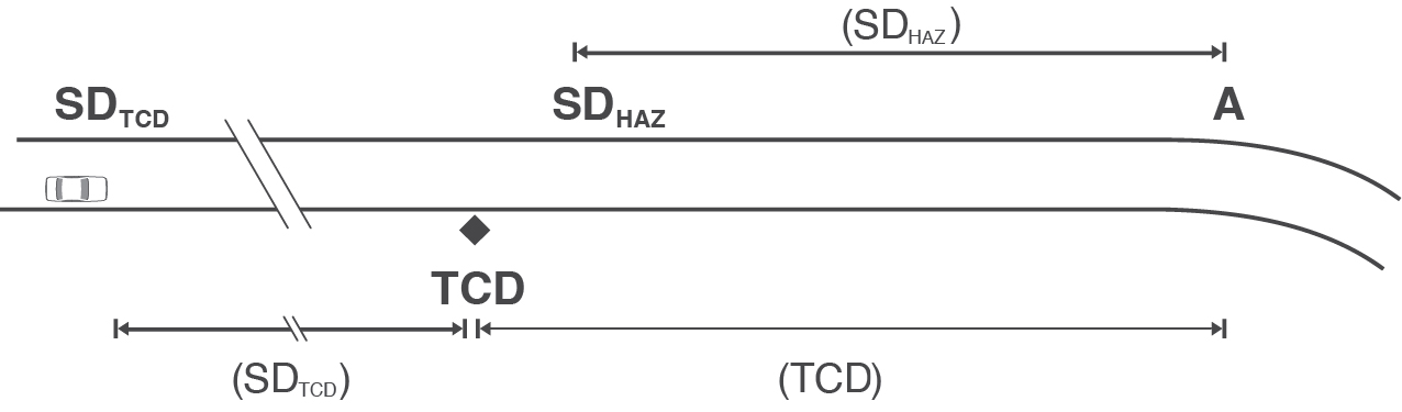
The illustration shows a segment between a car and a TCD on the side of the road, the segment is labeled SD TCD. A line segment below the road between the TCD and a curve in the road is labeled TCD. Above the road, a line segment labeled SD HAZ extends from points on the road labeled SD HAZ and A.
Step 2: Conduct Preliminary Engineering Analyses
This step involves the application of traditional traffic engineering techniques (e.g., AASHTO design policy geometric design criteria and DSD warrant) as a preliminary determinant of site deficiencies. In addition, the placement of traffic control devices needs to be examined in terms of MUTCD requirements.
Step 2A: Examine Hazard Location with Respect to AASHTO Design Criteria
Step 2B: Examine Approach with Respect to AASHTO Design Criteria
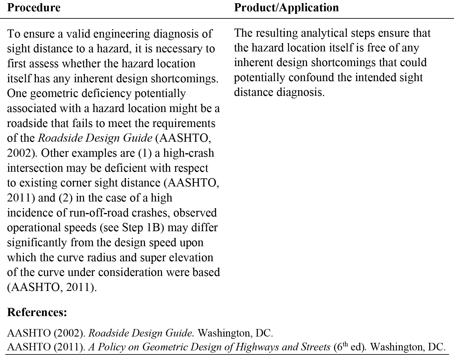
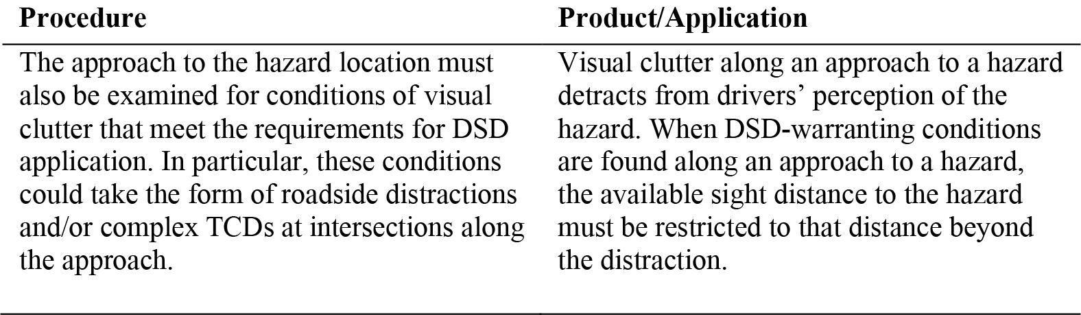
Step 2C: Examine Hazard Location with Respect to Possible DSD Warrants
![Procedure: AASHTO (2011) notes a distinction between typical stopping sight distances and those in which drivers are required to make complex decisions [i.e., in which drivers require P R T beyond the design value (typically 2.5 s)]. The D S D criterion applies to a difficult-to-perceive information source in a roadway environment that may be visually cluttered. Therefore, the hazard location needs to be examined for conditions of “visual noise” from competing sources of information (e.g., roadway elements, traffic, T C Ds, and advertising signs). Specific sources of visual clutter were also noted in Step 1E. Product / Application: hen D S D-warranting conditions are found, apply the sight distance requirements noted in AASHTO (2011) rather than conventional stopping distances based on a 2.5-s P R T.](https://www.nationalacademies.org/read/29158/assets/images/img_27-16_1.jpg)
Step 2D: Examine Approach with Respect to DSD Warrants
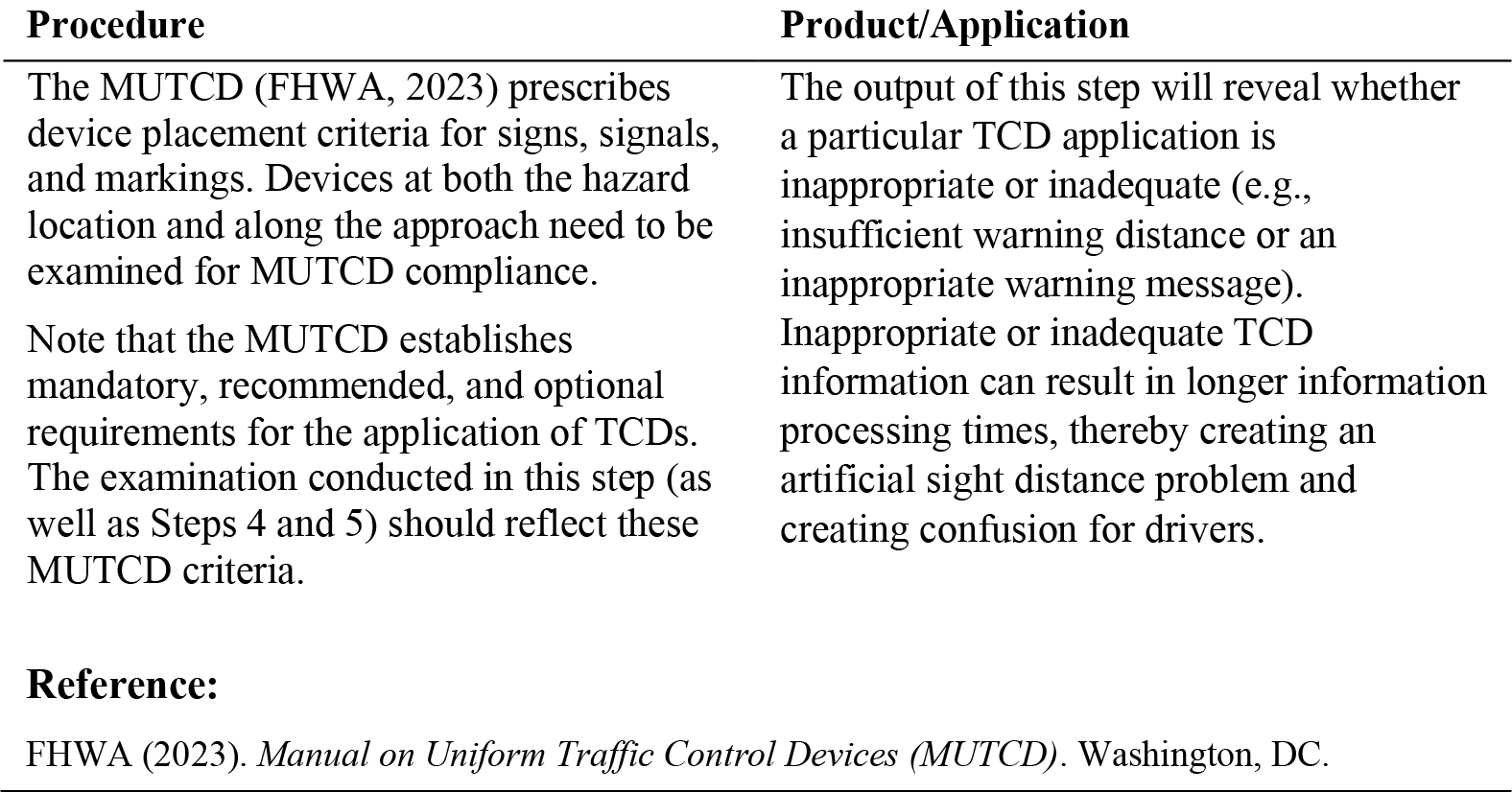
Step 2E: Examine Traffic Control Devices in Terms of MUTCD Criteria
Step 3: Apply Crash Data
This step involves integrating traffic crash data into the analysis. The objective is to identify specific crash-prone locations within the roadway segment, which may indicate sight distance problems. Note that the absence of crashes does not rule out the existence of a sight distance problem, as crashes are probabilistic events and reporting requirements are variable.
Step 3A: Establish Typologies and Frequency by Spot Locations
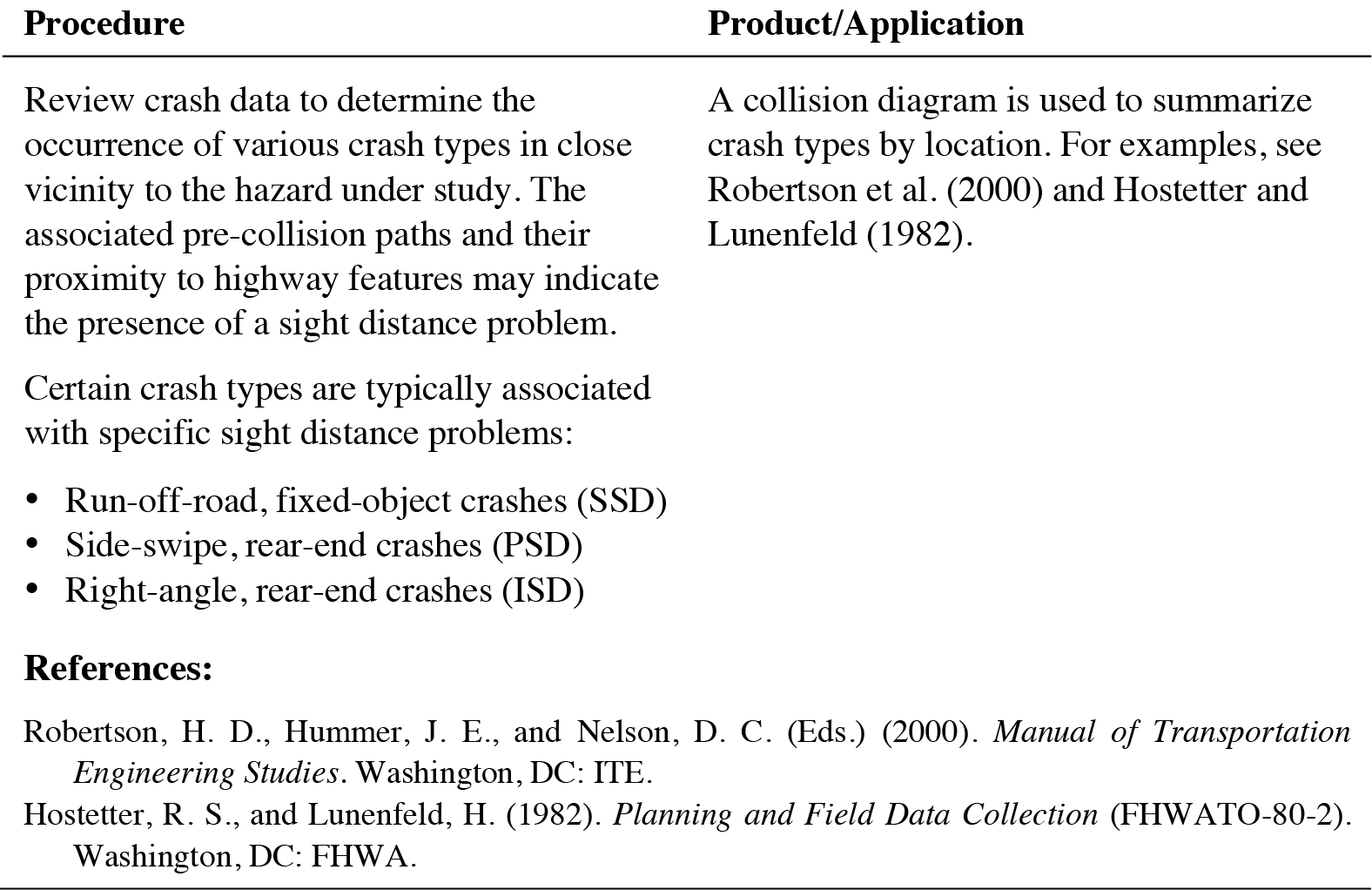
Step 3B: Assess Suitability of Crash Sample
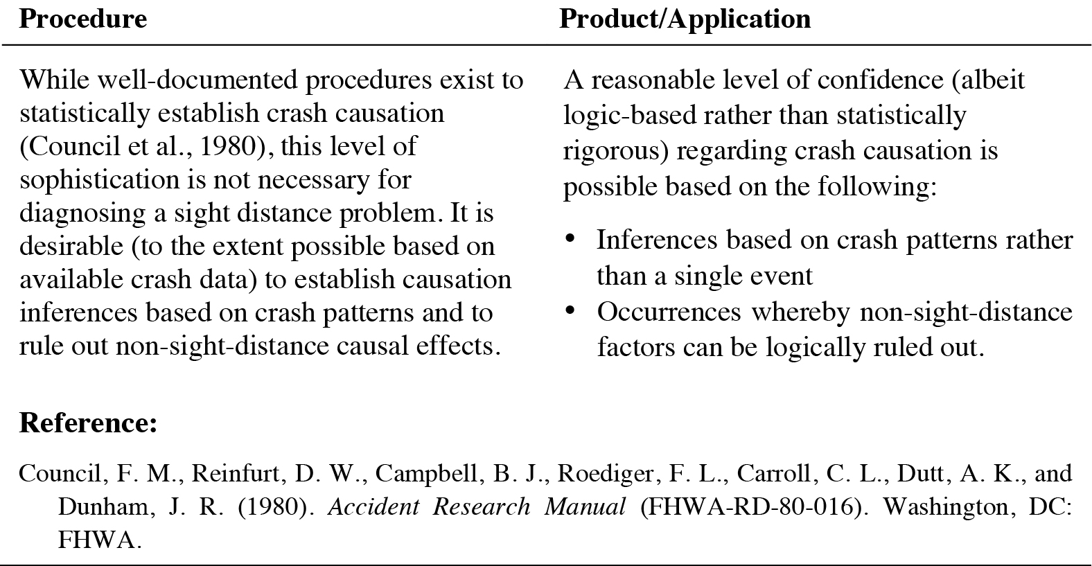
Step 3C: Examine Potential Sight Distance Causation Effect
Step 4: Establish Roadway Segments
The practitioner specifies component roadway approach segments in a manner to support the detailed human factors analysis in Step 5. Separate approach roadway segments are theoretically required for driver PRT and hazard avoidance maneuver functions. The product of this section is a series of driver task diagrams that depict the point where driver actions are required to avoid a potential hazard, as well as information sources that warn of the hazard and driversʼ available sight distances to perform the necessary information-processing and maneuver tasks.
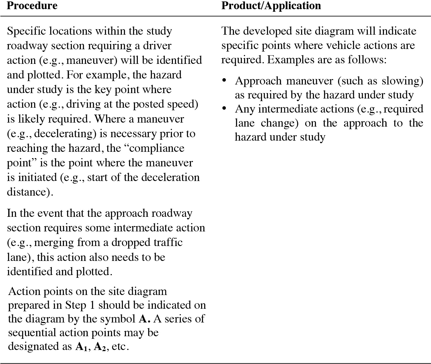
Step 4A: Establish and Plot Action Points Along Approach Segment
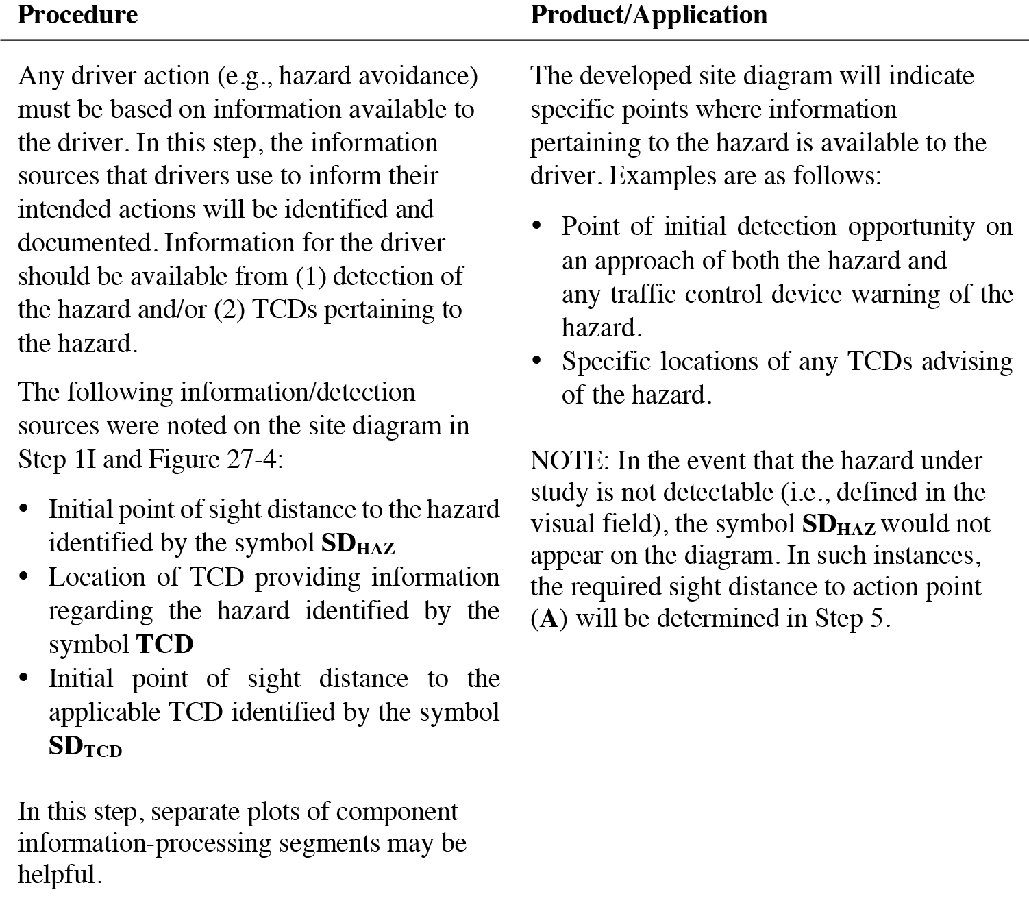
Step 4B: Establish and Plot Information Sources and Associated Sight Distances Along Approach Segment
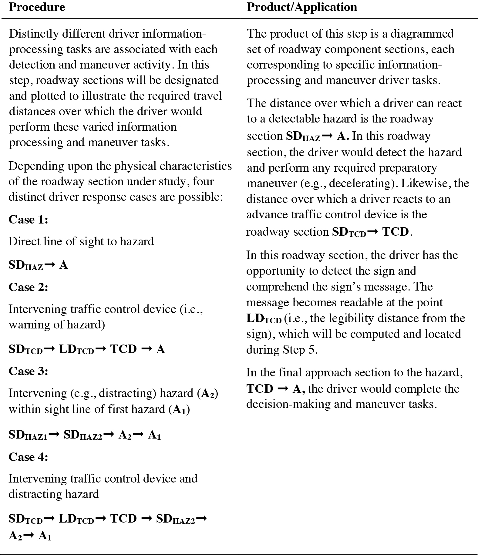
Step 4C: Define Component Driver Response Sections Within Approach Segment
Step 5: Analyze Component Driving Task Requirements
In this step, the practitioner applies human factors principles (comprising information-processing and decision-making criteria) to ensure the adequacy (or to quantify the shortcoming) of the approach roadway to allow for time/distance hazard avoidance requirements.
Step 5A: Determine the Relevant Geometric Design Sight Distance Application
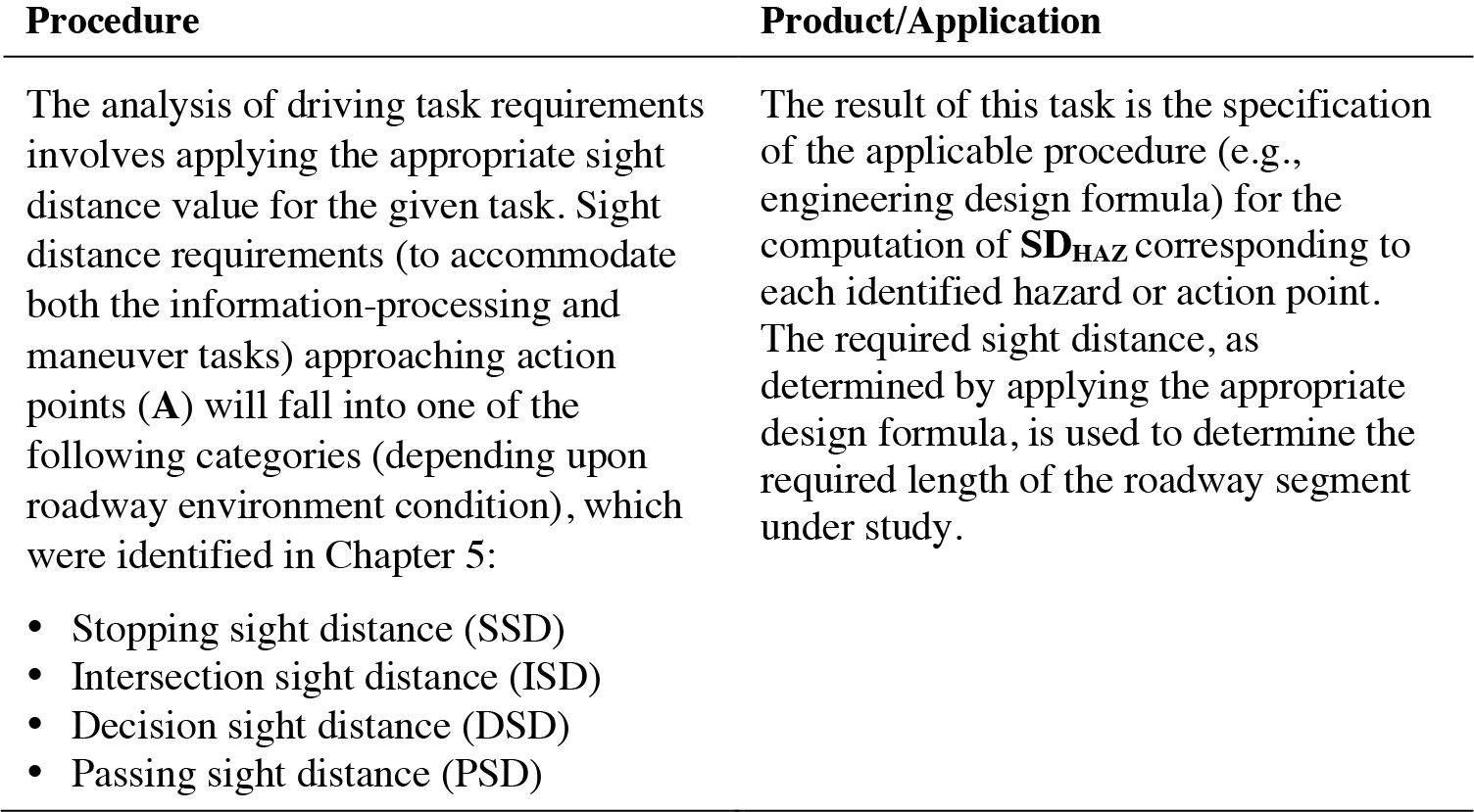
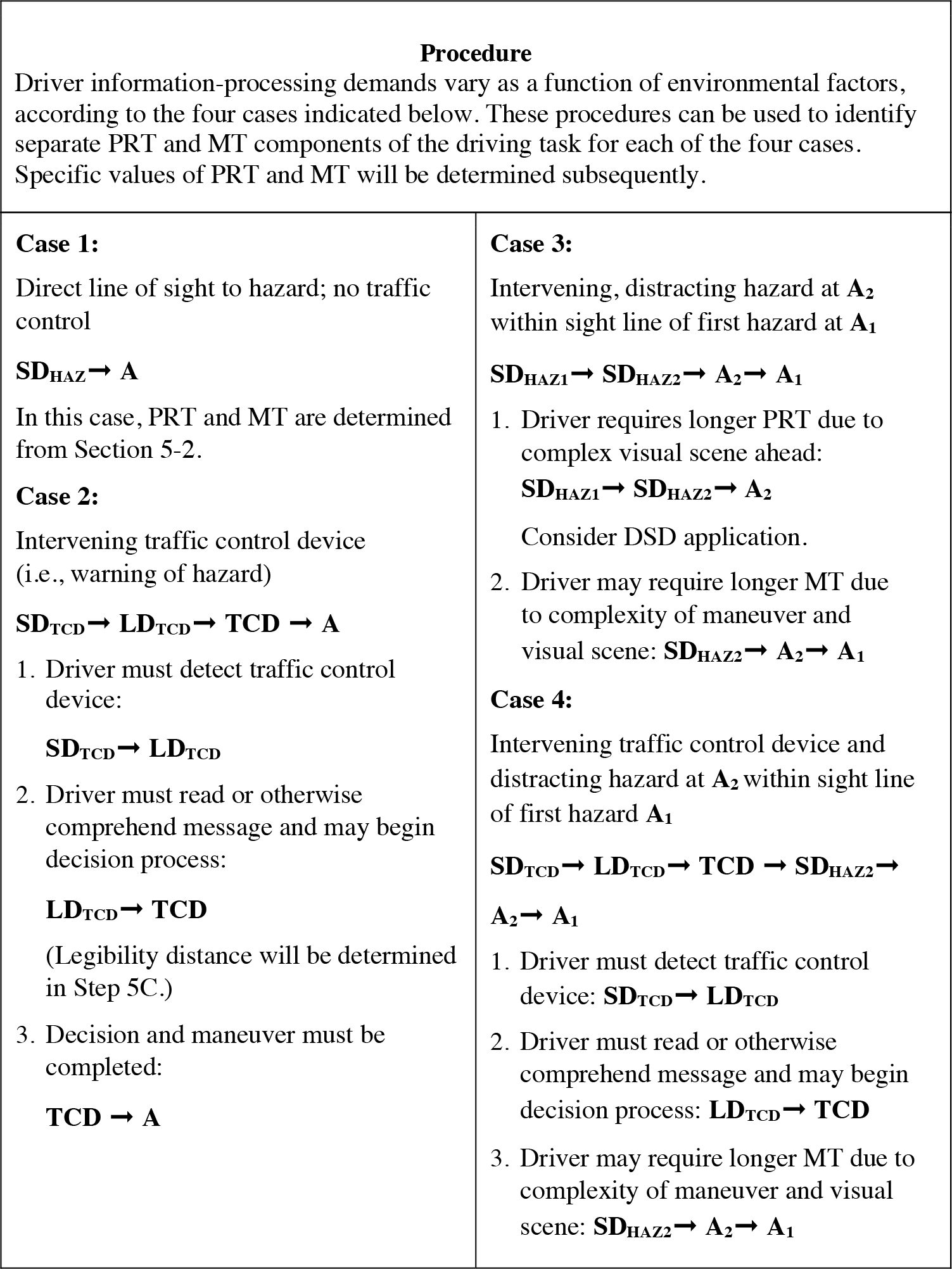
Step 5B: Determine Driving Task Requirements Within Each Component Roadway Segment
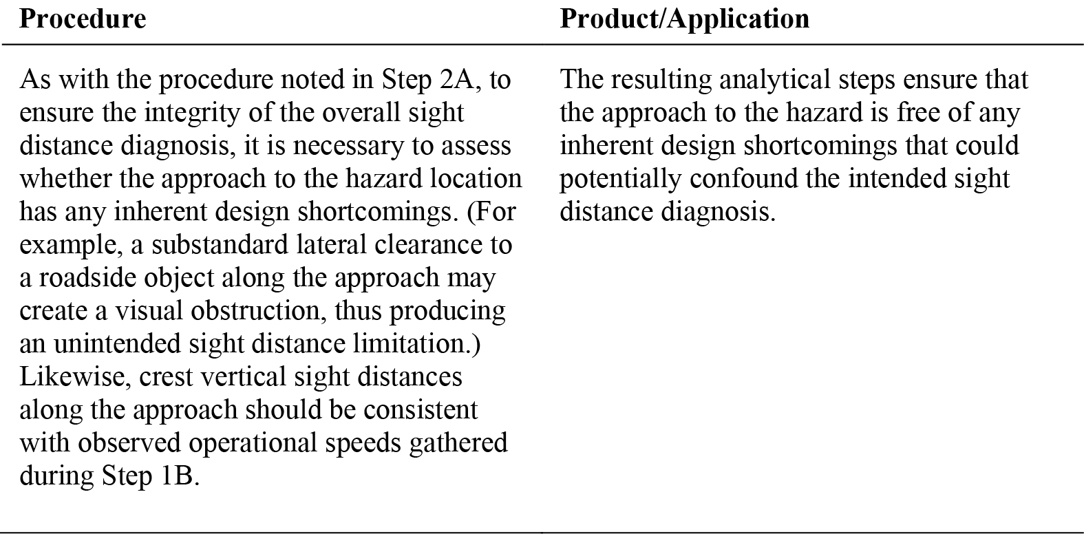
Step 5C: Quantify the Applicable PRT and MT Requirements for Each Driving Task Component
![Procedure: The general model to be applied for quantifying driver task requirements (i.e., required P R T and M T) is S D sub T C D➞ LD sub T C D➞ T C D ➞ A. Driver task requirements are determined for each task as follows. No T C Ds present: S D sub HAZ➞ A Apply applicable P R T and M T requirements corresponding to predetermined condition (i.e., S S D, IS D, D S D, or P S D as determined in Step 5A). T C Ds present: S D sub T C D➞ LD sub T C D Drivers should be able to detect a T C D prior to time required to comprehend its message; 2.5 s is desirable, although less time may be adequate (e.g., second, third, etc. in a sequence). LDT C D➞ T C D LDT C D is the “legibility distance” or approach distance at which a traffic control device message is comprehended. A detailed discussion in the following paragraphs addresses the LDT C D for signs. In the case of pavement markings, LDT C D is the advance distance at which the marking is visually recognized. The LDT C D for a sign is the distance at which its legend is read or its symbol message is comprehended. P R T requirements for signs consist of reading times for the message legend and symbol as follows (Smiley, 2000): Reading Time = 1*(number of symbols) + 0.5*(number of words and numbers) [s] The minimum reading time is 1 s. For messages exceeding four words, the sign requires multiple glances; the driver must look back to the road and at the sign again. Therefore, for every additional four words and numbers, or every two symbols, an additional 0.75 s should be added to the reading time. The LDT C D segment must be sufficient in length to accommodate the reading time noted above. However, its length is constrained by letter height (i.e., limited to 40 ft for every inch of letter height). For example, a 4-in. letter-height sign must be read within a distance of 4 × 40 = 160 feet. On a 40 mi/h (58.8 ft/s) roadway, the driver is limited to a maximum of 160/58.8 or 2.7 s to read the sign. Moreover, the traffic engineer must consider that the driver cannot be expected to fixate on the sign. Considering the driver’s alerted state after reading the sign, decision time (i.e., time to make a choice and initiate a maneuver if required) can range from 1 s for commonplace maneuvers (e.g., stop, reduce speed) to 2.5 s or more when confronted with a complex highway geometric situation. LD sub T C D➞ T C D ➞ A While the required M T may be initiated prior to passing the T C D, it must be completed in the above-noted segment. M T values associated with designed sight distance considerations are treated in Chapter 5. Additional literature sources with extensive maneuver time data are available (Lerner et al., 1999). References: Lerner, N. D., Steinberg, G. V., Huey, R. W., and Hanscom, F. R. (1999). Understanding Driver Maneuver Errors, Final Report (Contract DTFH61-96-C-00015). Washington, D C: F H W A. Smiley, A. (2000). Sign design principles. Ontario Traffic Manual. Ottawa, Canada: Ontario Ministry of Transportation.](https://www.nationalacademies.org/read/29158/assets/images/img_27-23.jpg)
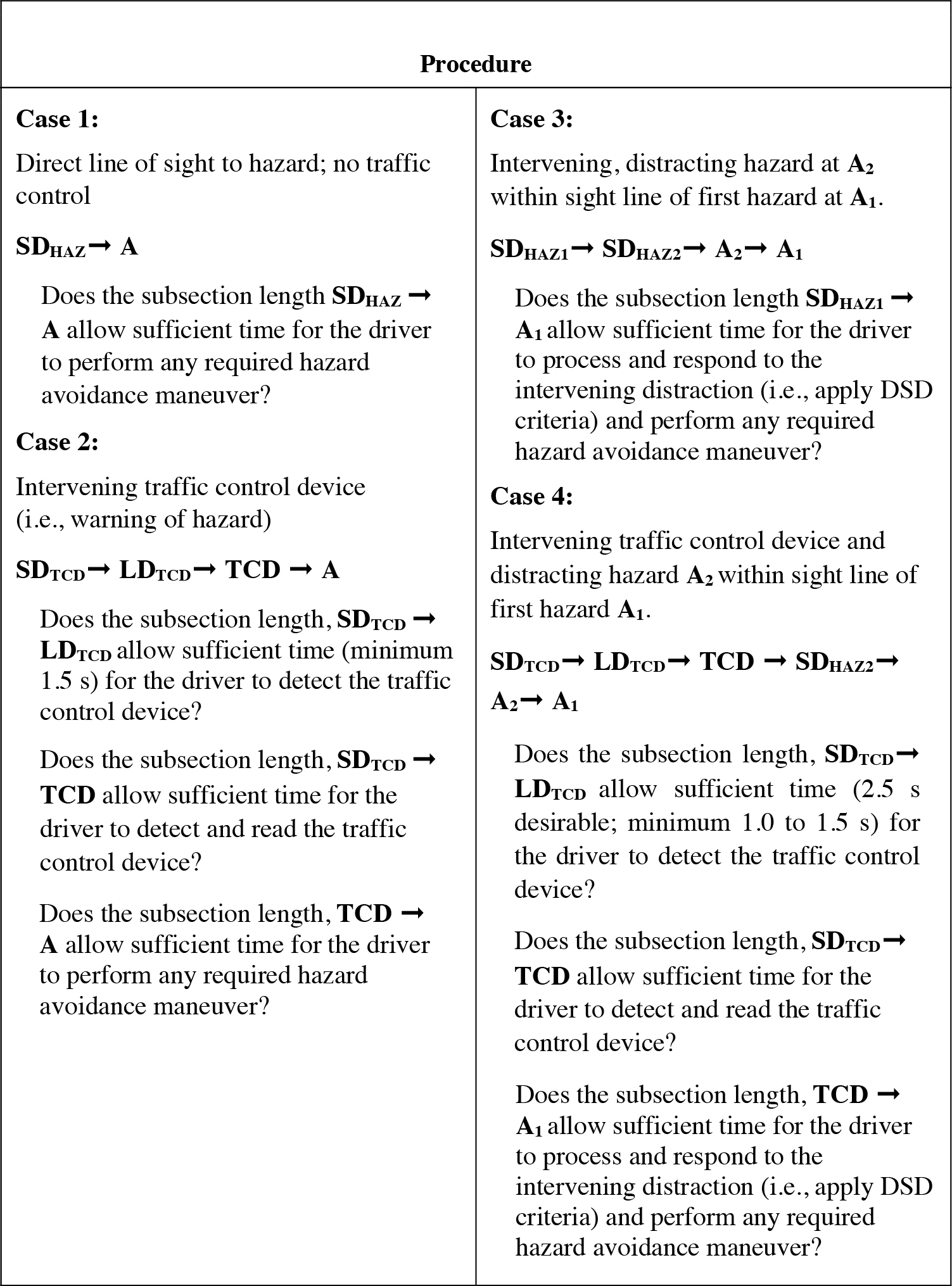
Step 5D: Assess the Adequacy of the Available Sight Distance Components
Step 6: Develop Engineering Strategies for Improvement of Sight Distance Deficiencies
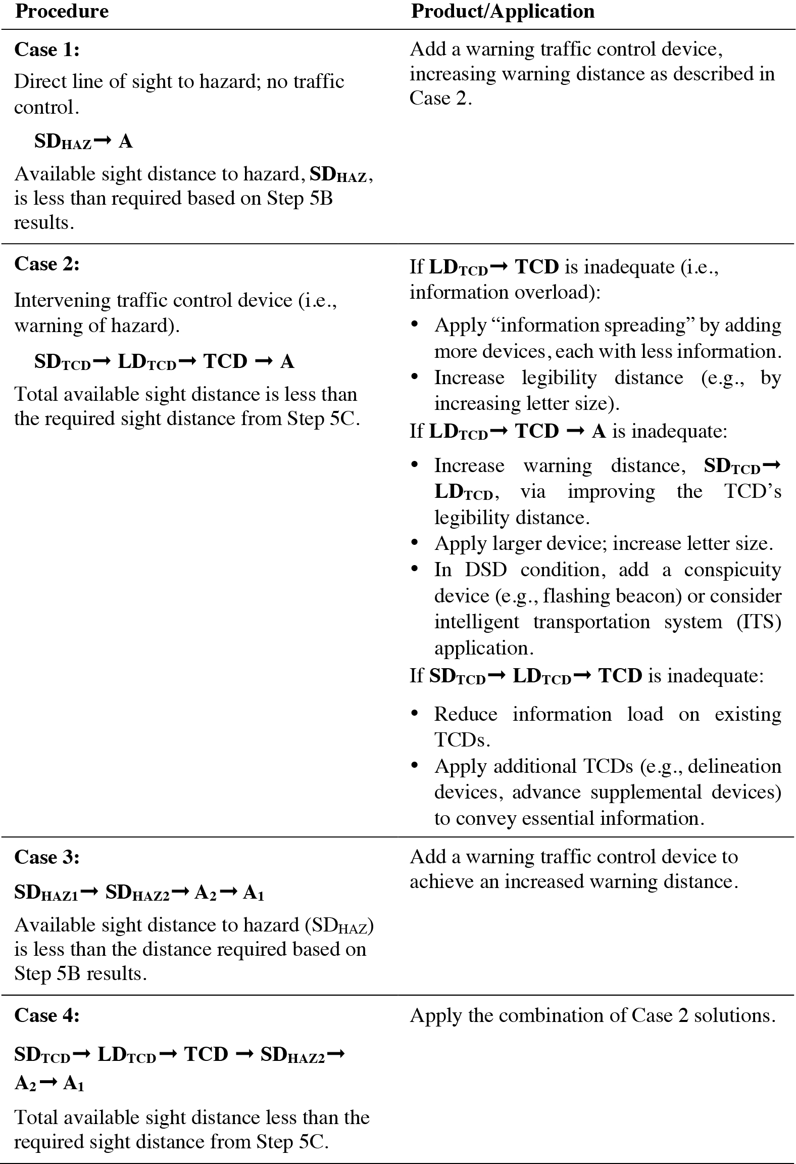
In this final step, the practitioner recommends improvement (e.g., traffic control device applications or minor design modifications) to correct deficiencies.
Step 6A: Apply Traffic Engineering and Highway Design Principles to Component Sight Distance Deficiencies
Example Application: Sight Distance Diagnostic Procedure
The example driving situation consists of a 55-mi/h, two-lane rural roadway that approaches a 35-mi/h curve followed by a stop-controlled intersection. The intersection approach is to a main highway, which requires the application of destination guide signing.
Driver requirements in this situation are as follows:
- Reduce speed from 55 to 35 mi/h to negotiate curve
- Process traffic control device information related to intersection (e.g., destination name sign)
- Stop for intersection
Step 1: Collect Field Data and Prepare Site Diagram
The labeled site diagram is shown in Figure 27-5.
Step 2: Conduct Preliminary Engineering Analyses
This example requires applying a sight distance analysis to two separate potential hazards. The first is a 35-mi/h curve that requires slowing from 55 mi/h; and the second is an intersection that is heavily signed with a stop sign and two guide signs, containing multiple route shields, symbols, and destination names. The approach roadways to each hazard point are separately treated as follows: (1) curve approach and (2) signed intersection approach.
Curve Approach Segment
Steps 2A through 2D: Examine Site with Respect to AASHTO Design Criteria and DSD Warrants. For the purpose of this example, it is assumed that geometrics conform to AASHTO and that DSD criteria (e.g., visually cluttered environmental conditions) do not apply.
Step 2E: Examine Traffic Control Devices for Compliance with the MUTCD. The MUTCD specifies requirements for warning signs. The curve warning sign in the example is a “W1-2, Horizontal Alignment Sign” with a 35-mi/h advisory speed plate. Section 2C-05 of the MUTCD
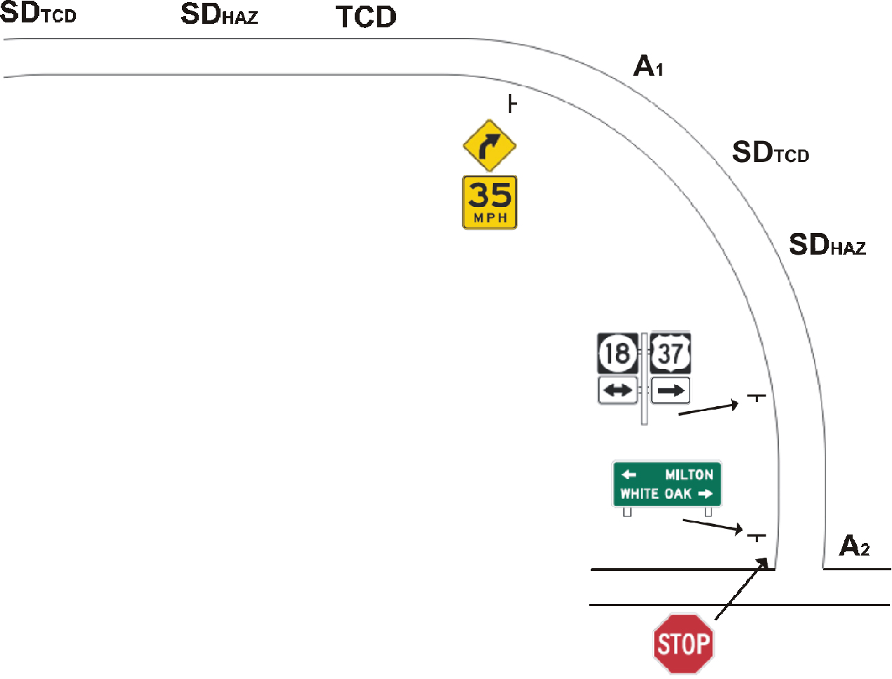
Long Description.
The approach to the curve has SD TCD, SD HAZ, and TCD labeled. At the beginning of the curve is a two-part road sign with a curved arrow and text reading 35 MPH. The curved segment of the road has the labels A1, SD TCD, and SD HAZ. As the curve ends, there are signs for route 18 in both directions and route 37 to the right, and a sign for Milton to the left and White Oak to the right. The intersection is labeled A2.
specifies an advance placement guideline for warning signs. Given the requirement to slow from 55 to 35 mi/h, the minimum recommended distance in Table 2C-4 is 138 ft (FHWA, 2003).
Signed Intersection Approach Segment
Steps 2A through 2D: Examine Site with Respect to AASHTO Design and DSD Criteria. For the purpose of this example, it is assumed that geometrics conform to AASHTO and that DSD criteria (e.g., visually cluttered environmental conditions) do not apply.
Step 2E: Examine Traffic Control Devices for Compliance with the MUTCD. This segment is a stop-controlled intersection approach containing signs to multiple routes and destinations.
The MUTCD provides requirements for guide signs on conventional roads. Signs in the example consist of a “directional assembly” with destination name signs and route shields. Required advance distances and spacing of these signs is given in Figure 2D-2 (FHWA, 2009). Typically, when a series of guide signs is placed sequentially along the approach to an intersection there is a 100- to 200-ft separation between the first two signs. The minimum spacing between signs is 100 ft, which is intended to enable drivers to read the entire message on both signs. Section 2D.06 requires 6-in. letter heights for a 35-mi/h roadway (FHWA, 2009).
Specifications for stop sign size and placement are contained in Chapter 2A of the MUTCD. As shown in Figure 2A-2 of the MUTCD, the stop sign should be set back a minimum of 12 ft from the intersection. The recommended letter height is 8 in. (FHWA, 2009).
Step 3: Apply Crash Data
Not conducted as part of this example.
Step 4: Establish Roadway Segments
This example requires a sight distance analysis of two separate potential hazards. The first is slowing from 55 mi/h to 35 mi/h, the posted curve advisory speed; and the second is a stop-controlled approach to an intersection containing signs to multiple routes and destinations. The approach roadways are discussed separately.
Curve Approach Segment
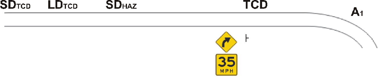
The roadway segment requiring the driver to slow from 55 mi/h to 35-mi/h is labeled in accordance with Steps 4A and 4B and is shown below. The two sight distance driver response scenarios follow:
- Case 1, direct line of sight to hazard (i.e., 55-mi/h speed zone to 35-mi/h curve): SDHAZ→A
- Case 2, intervening traffic control device (i.e., 35-mi/h advisory speed sign warning of hazard): SDTCD→LDTCD→TCD→A
This roadway is diagrammed in Figure 27-6.
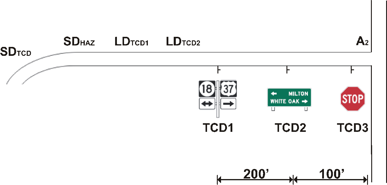
Signed Intersection Approach Segment
On this roadway section, motorists traveling at 35-mi/h are confronted with a stop-controlled intersection and two guide signs containing destination names and route shields. Because sight
Long Description.
The approach to the curve has labels for SD TCD, LD TCD, and SD HAZ, followed by a label for a sign with a curved arrow and text reading 35 MPH. A label next to the curve says A1.
distance to the intersection is limited by a curve on the approach, a sight distance analysis is critical. The component section diagram is labeled in accordance with Steps 4A and 4B and is shown below. The sight distance driver response scenarios follow:
- Case 1, direct line of sight to hazard (i.e., 35-mi/h speed zone to intersection): SDHAZ→ A
- Case 2: Three intervening traffic control devices
- A route shield assembly:
SDTCD1→ LDTCD1→ TCD1→ A - A destination name sign:
SDTCD2→ LDTCD2→ TCD2→ A - A stop sign:
SDTCD3→ LDTCD3→ TCD3→ A
- A route shield assembly:
This roadway segment is diagrammed in Figure 27-7.
Step 5: Analyze Component Driving Task Requirements
Curve Approach Segment
The analysis of component driving task requirements for this roadway section, which requires the driver to slow from a 55-mi/h speed zone to a 35-mi/h curve, considers sight distance to the curve and legibility distance requirements posed by the advisory speed sign.
Step 5A: Determine the Relevant Design Sight Distance Application. The applicable design sight distance is slowing sight distance—the required distance for a driver to observe the curve ahead and adjust speed accordingly. If certain visual noise conditions or other factors are present that would render the curve difficult to perceive, the practitioner must consider the applicable DSD criteria (discussed in Chapter 5). Where a traffic control device is present, driver information-processing time is required to observe and comprehend the sign, as well as slow to a safe curve negotiation speed. In the current example (i.e., a rural, uncluttered environment), DSD criteria are not applied.
Step 5B: Determine the Driving Task Requirements. Considering the two possibilities (i.e., Case 1 in which the driver observes the curve ahead without seeing the sign, and Case 2 in which the driver observes and comprehends the sign), the requirements for each are as follows:
- Case 1, direct line of sight to hazard (i.e., 55-mi/h speed zone to 35-mi/h curve): SDHAZ→ A
The sight distance requirement, in this case, is simply that the driver observes the curve ahead and slows to a safe speed.
Long Description.
The road begins with a curve and then straightens as it approaches a T intersection. The first label, next to the curve, is SD TCD. There are three labels above the road as it straightens: SD HAZ, LD TCD1, and LD TCD2. Below the road there are three labeled signs prior to the intersection: a pair of route signs that read 18 with arrows pointing both directions and 37 with an arrow pointing right; these are labeled TCD1. Next, a sign reading Milton with an arrow pointing left and White Oak with an arrow pointing right; this is labeled TCD2. Next, a stop sign, labeled TCD3. A label above the road at the intersection reads A2.
- Case 2, intervening traffic control device (i.e., 35-mi/h advisory speed sign warning of hazard):
SDTCD→ LDTCD→ TCD → A
The sight distance requirement in this case is that the driver observes the sign, comprehends the sign message, and slows to a safe speed.
Step 5C: Quantify the Applicable PRT and MT Requirements for Each Driving Task.
- Case 1, direct line of sight to hazard (i.e., 55-mi/h speed zone to 35-mi/h curve): SDHAZ→ A
Because DSD does not apply (as determined in Step 5A), the design PRT value of 2.5 s is applied; thus, the PRT component of sight distance is 202 ft (i.e., 2.5 s times 80.85 ft/s). The MT requirement (4.0 s) is derived from the need to slow from 55 mi/h to 35 mi/h at a comfortable deceleration level (i.e., .23g), which requires 261 ft. Thus, the total PRT and MT sight distance requirement is 463 ft.
The comfortable deceleration level is derived from Table 2-25 of AASHTO (2011a). (For safety purposes, wet weather deceleration is considered.) However, AASHTO (2011a) acknowledges that its deceleration data may be outdated and that more rapid (albeit uncomfortable) decelerations are common. A typical such deceleration is 0.35g (Knipling et al., 1993), resulting in an MT of 2.6 s. It is also known that most reasonably alert drivers can initiate braking with a PRT of 1.6 s (see page 5-4, “Determining Stopping Sight Distance”). Applying these performance parameters to slowing from 55 mi/h to 35 mi/h, the total required PRT distance is 129 ft plus 172 ft MT distance, or 301 ft.
It is unlikely that the need to slow to 35 mi/h would be visually evident from an advance distance of either 301 or 463 ft. Therefore, the critical sight distance consideration is based on the application of the speed advisory sign. - Case 2, intervening traffic control device (i.e., 35-mi/h advisory speed sign warning of hazard):
SDTCD→ LDTCD→ TCD → A
In this case, the driver needs to detect the sign, read the sign, and decelerate to a safe speed for the curve. A critical requirement for sight in advance of a sign (i.e., allowing time to comprehend the signʼs message) is known as legibility distance. There is a considerable body of knowledge regarding sign legibility distance requirements (Smiley, 2000).
For simple warning signs, the MUTCD specifies an advance placement guideline, which includes “an appropriate legibility distance” of 175 ft for word legend signs or 100 ft for symbol signs. The MUTCD sign placement requirement to allow for slowing from 55 to 35 mi/h is 350 ft (FHWA, 2009).
Driver requirements imposed by the MUTCD rule in this case are as follows: Given that 2.0 s are needed to detect and comprehend (e.g., minimum 1.0 s for detection plus 1.0 s for symbol comprehension) the simple warning sign message prior to the initiation of slowing, the deceleration requirement would be .32g or approximately the equivalent slowing rate of skidding on wet pavement (FHWA, 2009). In this example, the required PRT and MT distances would be 161 and 189 ft, respectively, for a total of 350 ft.
For signs with complex messages (i.e., sets of destination names or symbols in combination with symbols), message comprehension may require significantly more legibility distance. The next example illustrates such a situation.
Signed Intersection Approach Segment
On this roadway section, motorists traveling at 35 mi/h are confronted with a stop-controlled intersection and two guide signs containing destination names and route shields. Because sight distance to the intersection is limited by a curve on the approach, a sight distance analysis is critical.
Step 5A: Determine the Relevant Design Sight Distance Application. As the driver approaches a stop-controlled intersection, there must be sufficient available SSD (Chapter 5) to enable
stopping at the stop line. (While the negotiation of the intersection involves the application of ISD, the current example is limited to approaching the intersection.)
Step 5B: Determine the Driving Task Requirements. Considering the two possibilities (i.e., Case 1 in which the driver proceeds to the intersection ahead while ignoring the signs, and Case 2 whereby the driver observes and comprehends the intermediate signs), the requirements are as follows:
- Case 1, direct line of sight to hazard (i.e., 35-mi/h speed zone to intersection): SDHAZ→ A
The sight distance requirement (to accommodate travel time), in this case, is simply that the driver observes the intersection ahead and safely slows to a stop. - Case 2, three intervening traffic control devices, i.e.:
- A route shield assembly:
SDTCD1→ LDTCD1→ TCD1→ A - A destination name sign:
SDTCD2→ LDTCD2→ TCD2→ A - A stop sign:
SDTCD3→ LDTCD3→ TCD3→ A
The sight distance requirement in this case is that the driver detects and comprehends the signs and slows to a safe stop at the stop line. - A route shield assembly:
Step 5C: Quantify the Applicable PRT and MT Requirements for Each Driving Task
- Case 1, direct line of sight to hazard (i.e., speed reduction from 35 mi/h to stop at the stop line): SDHAZ→ A
The design SSD does not accommodate the information-processing requirements of the intervening guide signs. The AASHTO design SSD value (AASHTO, 2004) for a 35-mi/h approach is 225 to 250 ft, which accounts for both the PRT and MT tasks.
However, this 225- to 250-ft sight distance would barely accommodate the physical placement of the two guide sign assemblies that are shown in Figure 27-7. Moreover, the information processing load imposed by the signs requires significant attention and, therefore, higher sight distance requirements. Case 2 describes how to determine sight distance requirements for these conditions. - Case 2, intervening traffic control device (i.e., guide signs): SDTCD→ LDTCD→ TCD → A
This general model entails the following considerations. First, there must be sufficient sight distance so that the sign is detected prior to the time required to comprehend the signʼs message, thus application of the SDTCD term. This advance distance is not specified in the MUTCD. Nevertheless, 2.5 s is desirable for this sign detection task, although less time may be adequate as motorists who are looking for signs are generally aware of the expected position in their field of view. The more essential approach sight distance to a traffic control device is that required to comprehend its message.
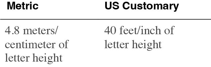
LDTCD refers to legibility distance—the approach distance at which a TCD legend is read or its symbol message is comprehended. The legibility distance of a legend sign is determined by multiplying a legibility index (i.e., the distance at which a given unit of letter height is readable) by the letter height. The applicable legibility index values are shown in Table 27-2. For example, the legibility distance typically associated with 6-in. letter height is 240 ft (40 times 6).
The legibility distance of symbol signs has been investigated in a laboratory study (Dewar et al., 1994) and found to significantly exceed that of legend signs, despite the high degree of
Long Description.
The Metric legibility index value is 4.8 meters per centimeter of letter height. The US Customary legibility index is 40 feet per inch of letter height.
variability in the study data. For example, the mean legibility distance for the right curve arrow symbol was determined to be 283 m (with a standard deviation of 68 m). Considering that a 55-mi/h approach allowing a 2.5-s advance sight distance and 1.0-s reading time would consume only 86 m, pure symbol signs are not expected to result in an information-processing problem.
The required PRT for this example roadway segment consists of three components: sign detection, sign comprehension, and intersection detection.
Sign Detection. Upon a driverʼs detection of the first sign, the second and third signs would require minimal detection time. The recommended detection time for the first sign is 2.5 s; however, the second two signs are likely to be detected much more rapidly. “Alerted” PRT responses are known to occur in as little as 1.0 to 1.5 s. Moreover, signs can be quickly detected as drivers know where to look for signs and typically scan toward expected sign locations. Therefore, a conservative sign detection PRT for the example roadway segment is (2.5 + 1.5 + 1.5) or 5.5 s.
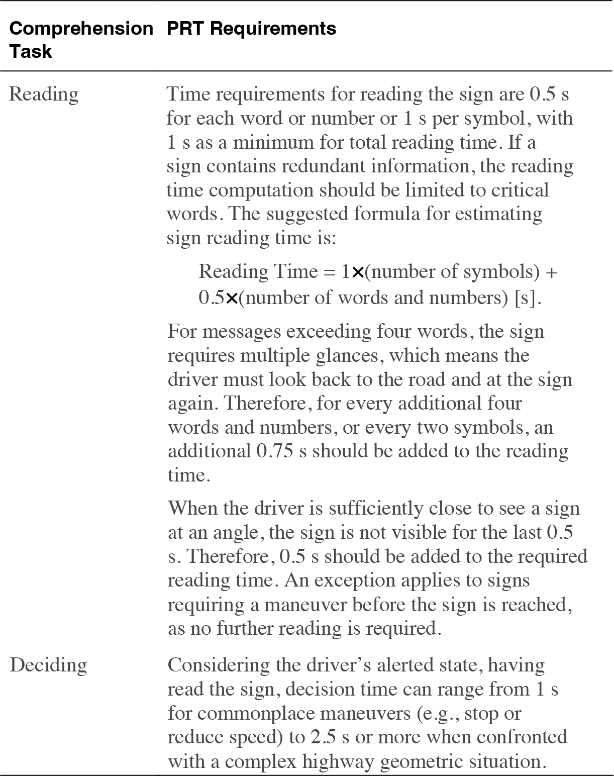
Sign Comprehension. Sign comprehension consists of reading the sign plus making the resultant decision (e.g., right or left turn in response to the signʼs information). The PRT requirement (Smiley, 2000) is based on sign-response reading and decision time, for which general rules are noted in Table 27-3.
The first guide sign assembly contains two numbers and two symbols, requiring 3.0 s of reading time; the second contains two designation names and two symbols, also requiring 3.0 s; and the third is a simple and familiar one-word regulatory sign, requiring 1 s. Thus, the total sign reading time is 7.0 s. This estimate is highly conservative, as drivers would likely scan the guide signs seeking only a particular name or route number; however, it is necessary to provide sufficient information-processing sight as some drivers may need the entire set of information. An additional 3.0 s is considered for decision time responses to the three signs. Thus, the total comprehension time for the three signs is 10 s.
Intersection Detection Distance. As noted above under the Case 1 (SDHAZ→A) discussion, the SSD requirement considers a 2.5-s PRT.
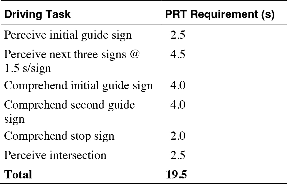
A summary of these PRT requirements, broken down in terms of separate driving tasks, is shown in Table 27-4. The sum of PRT requirements would apply to a serial task process. However, a realistic assessment of PRT requirements considers that many of the tasks in Table 27-4 are concurrent. For example, comprehending the stop sign would not necessarily be separate from perceiving the intersection, thus potentially reducing the total PRT by 2.5 s. In addition, following a driverʼs 2.5-s detection of the initial sign, the subsequent two signs would likely be detected with a minimum detection time (e.g., 1.0 s rather than 1.5 s), thus conceivably reducing the total PRT by another 1.0 s. Therefore, subtracting 3.5 s from the serial total of 19.5 s, the estimated PRT requirement becomes 16.0 s.
The MT requirement (i.e., to slow from 35 mi/h to a stop at the specified AASHTO g-force) calculates to 4.7 s over a distance of 120 ft. The extent to which the deceleration process would occur concurrently with the various sign-response tasks is uncertain. However, it is logical (and best serves liability concerns) to allow time for comprehension of all signs prior to the initiation of the slowing response.
Long Description.
The table provides PRT requirements for two comprehension tasks: reading and deciding. The PRT requirements for reading are as follows: Time requirements for reading the sign are 0.5 s for each word or number or 1 s per symbol, with 1 s as a minimum for total reading time. If a sign contains redundant information, the reading time computation should be limited to critical words. The suggested formula for estimating sign reading time is: Reading Time = 1×(number of symbols) + 0.5×(number of words and numbers) [s]. For messages exceeding four words, the sign requires multiple glances, which means the driver must look back to the road and at the sign again. Therefore, for every additional four words and numbers, or every two symbols, an additional 0.75 s should be added to the reading time. When the driver is sufficiently close to see a sign at an angle, the sign is not visible for the last 0.5 s. Therefore, 0.5 s should be added to the required reading time. An exception applies to signs requiring a maneuver before the sign is reached, as no further reading is required. The PRT requirements for Deciding are as follows: Considering the driver’s alerted state, having read the sign, decision time can range from 1 s for commonplace maneuvers (e.g., stop or reduce speed) to 2.5 s or more when confronted with a complex highway geometric situation.
Long Description.
The table provides PRT requirement values (in seconds) for 6 driving tasks, and also provides the total PRT requirement for the 6 tasks. Perceive initial guide sign: 2.5. Perceive next three signs at 1.5 seconds per sign: 4.5. Comprehend initial guide sign: 4.0. Comprehend second guide sign: 4.0. Comprehend stop sign: 2.0. Perceive intersection: 2.5. Total: 19.5.
Long Description.
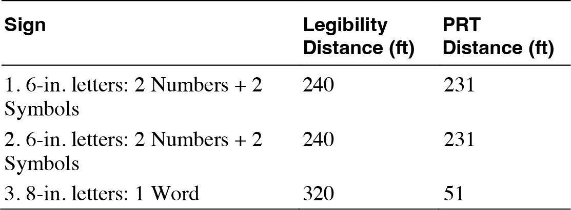
For signs that have 6-inch letters, 2 numbers and 2 symbols, the legibility distance is 240 feet and the PRTdistance is 231 feet. For signs that have 8-inch letters and 1 word, the legibility distance is 320 feet and the PRT distance is 51 feet.
Therefore, the overall sight distance requirement is approximately 16.0 s of sign information processing at 35 mi/h (51.45 ft/s) or 823 ft, plus the 120-ft deceleration distance, for a total of 943 ft. Actual requirements will reflect real-world conditions. If possible, data should be collected at the relevant sites.
A final consideration is the necessity that drivers have sufficient time to comprehend a signʼs message during the interval when the message is discernable. Therefore, an essential sight distance diagnostic step is to compare the available sign legibility distance (i.e., available reading distance) with the distance traveled during reading PRT (i.e., required reading distance and decision time). Table 27-5 contrasts the distance traveled during PRT with the legibility distance. While the guide signs in this example accommodate both reading time and associated decision time, the decision component of PRT can obviously be accomplished after the driver passes the sign.
Step 6: Develop Engineering Strategies for Improvement of Sight Distance Deficiencies
Not conducted as part of this example.
Tutorial 3: Detailed Task Analysis of Curve Driving
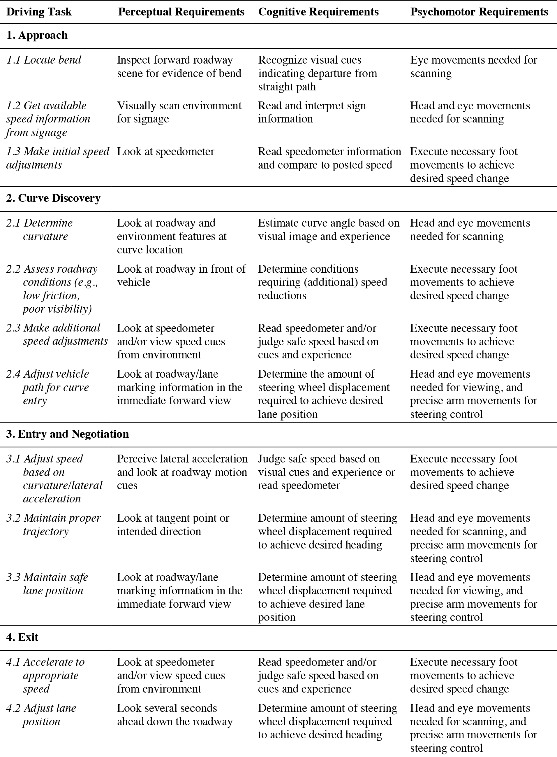
This tutorial presents a task analysis of the different activities that drivers must conduct while approaching and driving through a single curve (with no other traffic present) to provide qualitative information about the various perceptual, cognitive, and psychomotor elements of curve driving. Consistent with established procedures for conducting task analyses (Campbell and Spiker, 1992; Richard, Campbell, and Brown, 2006; McCormick, 1979; Schraagen, Chipman, and Shalin, 2000), the task analysis was developed using a top-down approach that successively decomposed driving activities into segments, tasks, and subtasks. The approach used in this tutorial was specifically based on the one described in Richard, Campbell, and Brown (2006); readers interested in additional details about the methodology should consult that reference.
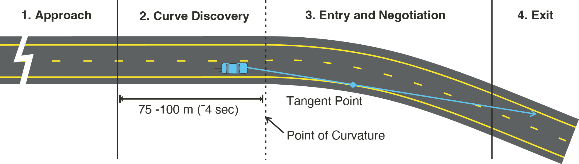
The curve-driving task was broken down into four primary segments, with each segment generally representing a related set of driving actions (Figure 27-8). The demarcation into segments was primarily for convenience of analysis and presentation and does not imply that the curve-driving task can be neatly carved up into discrete stages. Within each segment, the individual tasks that drivers must perform to navigate the curve safely were identified. Moreover, these driving tasks were further divided based on the information-processing elements (perceptual, cognitive, and psychomotor) necessary to adequately perform each task. The perceptual requirements typically refer to the visual information about the curve and the surrounding roadway needed to judge the curvature, determine lane position and heading, etc. The cognitive requirements typically refer to the evaluations, decisions, and judgments that drivers must make about the curve or the driving situation. The psychomotor requirements refer to the control actions (e.g., steering wheel movements, foot movements to press brake) that drivers must make to maintain vehicle control or to facilitate other information acquisition activities.
The task analysis presented in Table 27-6 shows the driving tasks and corresponding information-processing subtasks associated with driving a typical horizontal curve approaching from a long tangent. Drivers must also engage in other ongoing safety-related activities, such as scanning the environment for hazards; they may also engage in in-vehicle tasks such as adjusting the radio, using windshield wipers, or consulting a navigation system (just to name a few). However, these more generic tasks are not included in the task analysis to emphasize those tasks and subtasks that are directly related to curve driving.
The primary source of information for segment tasks was the comprehensive driving task analysis conducted by McKnight and Adams (1970); however, other research more specifically related to curve driving was also used, including Donges (1978), Fitzpatrick et al. (2000), Groeger (2000), Krammes et al. (1995), McKnight and Adams (1970), Pendleton and Messer (1995), Richard et al. (2006), Salvendy (1997), Serafin (1994), Underwood (1998), and Vaniotou (1991).
Long Description.
The approach segment of the road has a jagged line through it. The curve discovery segment is labeled as having length of 75 to 100 meters (~ 4 seconds). A car is shown near the end of this segment, with a blue arrow extending forward from it. At the end of the curve discovery segment is a dashed line labeled the point of curvature. The road begins to curve at the entry and negotiation segment. A dot along the blue arrow extending from the car is labeled tangent point. The arrow extends into the Exit segment.
Long Description.
The table has 4 columns. The column headings are as follows: Column 1: Driving Task. Column 2: Perceptual Requirements. Column 3: Cognitive Requirements. Column 4: Psychomotor Requirements. The table is divided into 4 sections: 1. Approach, 2. Curve Discovery, 3. Entry and Negotiation, 4. Exit. The data rows for section 1: Approach are as follows: Row 1.1. Column 1: Locate Bend. Column 2 Inspect forward roadway scene for evidence of bend. Column 3: Recognize visual cues indicating departure from straight path. Column 4: Eye movements needed for scanning. Row 1.2, Column 1: Get available speed information from signage. Column 2: Visually scan environment for signage. Column 3: Read and interpret sign information. Column 4: Head and eye movements needed for scanning. Row 1.3, Column 1: Make initial Speed adjustments. Column 2: Look at speedometer. Column 3: Read speedometer information and compare to posted speed. Column 4: Execute necessary foot movements to achieve desired speed change. The data for section 2: Curve Discovery are as follows: Row 2.1,Column 1: 2.1 Determine curvature Column 2: Look at roadway and environment features at curve location Column 3: Estimate curve angle based on visual image and experience Column 4: Head and eye movements needed for scanning Row 2.2 Column 1 Assess roadway conditions (e.g., low friction, poor visibility) Column 2 Look at roadway in front of vehicle Column 3: Determine conditions requiring (additional) speed reductions Column 4: Execute necessary foot movements to achieve desired speed change Row 2.3 Column 1: Make additional speed adjustments Column 2: Look at speedometer and/or view speed cues from environment Column 3: Read speedometer and/or judge safe speed based on cues and experience Column 4: Execute necessary foot movements to achieve desired speed change Row 2.4, Column 1: Adjust vehicle path for curve entry Column 2: Look at roadway/lane marking information in the immediate forward view Column 3: Determine the amount of steering wheel displacement required to achieve desired lane position Column 4: Head and eye movements needed for viewing, and precise arm movements for steering control The data for section 3, Entry and Negotiation are as follows: Row 3.1 Column 1 Adjust speed based on curvature/lateral acceleration Column 2: Perceive lateral acceleration and look at roadway motion cues Column 3: Judge safe speed based on visual cues and experience or read speedometer Column 4: Execute necessary foot movements to achieve desired speed change Row 3.2, Column 1: Maintain proper trajectory Column 2 Look at tangent point or intended direction Column 3 Determine amount of steering wheel displacement required to achieve desired heading Column 4 Head and eye movements needed for scanning, and precise arm movements for steering control Row 3.3 Column 1 Maintain safe lane position Column 2: Look at roadway/lane marking information in the immediate forward view Colum 3: Determine amount of steering wheel displacement required to achieve desired lane position Column 4: Head and eye movements needed for viewing, and precise arm movements for steering control The data for section 4: Exit are as follows: Row 4.1 Row 4.1 Column 1: Accelerate to appropriate speed Column 2: Look at speedometer and/or view speed cues from environment Column 3: Read speedometer and/or judge safe speed based on cues and experience Column 4: Execute necessary foot movements to achieve desired speed change Row 4.2 Column 1: Adjust lane position Column2: Look several seconds ahead down the roadway Column 3: Determine amount of steering wheel displacement required to achieve desired heading Column 4: Head and eye movements needed for scanning, and precise arm movements for steering control
For the most part, these references and the other research provided information about which tasks were involved in a given segment, but not complete information about the specific information-processing subtasks. To determine this information, the details about the information-processing subtasks and any other necessary information were identified by the authors based on expert judgment and other more general sources of driving behavior and human factors research (e.g., Groegor, 2000; Salvendy, 1997; Underwood, 1998).
Tutorial 4: Determining Appropriate Clearance Intervals
Methods for determining appropriate clearance interval length vary from agency to agency, and there is no consensus on which is the best method. The Institute of Transportation Engineers recommends several procedures for determining clearance interval duration in a 1994 informational report (see ITE, 1994) on signal change interval lengths. These methods include:
- A rule of thumb based on approach speed, such as this one presented in the ITE Traffic Engineering Handbook (Pline, 1999):
- Yellow change time in seconds = operating speed in mi/h/10
- Red clearance interval = 1 or 2 s
- Formulas for calculating interval lengths based on site, vehicle, and human factors characteristics, such as this equation (from Pline, 1999):
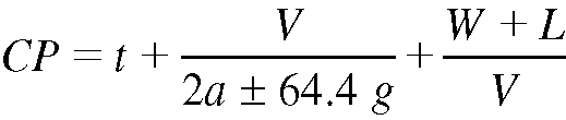
Long Description.
CP equals t plus start fraction V over 2 a plus 2 G g end fraction plus start fraction W plus L over V end fraction
Where:
CP = non-dilemma change period (change + clearance intervals)
t = perception-reaction time (nominally 1 s)
V = approach speed m/s [ft/s]
g = percent grade (positive for upgrade, negative for downgrade)
a = deceleration rate (m/s2) (typical 3.1 m/s2) [typical 10 ft/s2]
W = width of intersection, curb to curb (m) [ft]
L = length of vehicle (typical 6 m) [typical 20 ft]
- A uniform clearance interval length—Various studies report that uniform value of 4 or 4.5 s for the yellow change interval length throughout a jurisdiction is sufficient to accommodate most approach speeds and deceleration rates. Refer to Determining Vehicle Signal Change and Clearance Intervals (ITE, 1994) for more discussion on this.
The MUTCD (FHWA, 2023b) states that a yellow change interval should be approximately 3 to 6 s, and the Traffic Engineering Handbook (Pline, 1999) states that a maximum of 5 s is typical for the yellow change interval. The red clearance interval, if used, should not exceed 6 s (FHWA, 2023b), but 2 s or less is typical (Pline, 1999). The traffic laws in each state may vary from these suggested practices. ITE recommends that the yellow interval not exceed 5 s, so as not to encourage driver disrespect for signals.
Tutorial 5: Determining Appropriate Sign Placement and Letter Height Requirements
When determining the appropriate sign placement, it is important to consider a number of driver-related factors. The Traffic Control Devices Handbook (Pline, 2001) describes a process that utilizes these factors and is the basis for the steps described below. This method is mostly focused on guide and informational sign applications.
Step 1. Calculate the Reading Distance
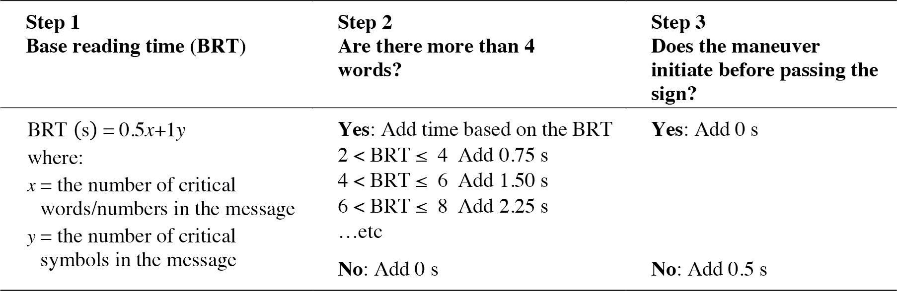
The reading distance is the portion of the traveling distance allotted for the driver to read the message, based upon the time required to read it (reading time). The Traffic Control Devices Handbook (Pline, 2001) outlines two methods for calculating the reading time. The first method, used by the Ontario Ministry of Transportation Traffic Office (2001), is described in the following three steps:
- Allocate 0.5 s per word or number and 1 s per symbol, with a 1-s minimum for the total reading time. This time should only include critical words. Drivers do not need to read every word of each destination listed on a sign to find the one they are looking for. For example, assume they are reading a sign with two destinations: Mercer St. and Union St., each with a direction arrow. Drivers only need to read the word Mercer to realize that it is not the street they are looking for and the word Union to know that is their destination. They then only need to look at the arrow for Union St.
- “If there are more than four words on a sign, a driver must glance at it more than once, and look back to the road and at the sign again. For every additional four words and numbers, or every two symbols, an additional 0.75 s should be added to the reading time” (Ontario Ministry of Transportation Traffic Office, 2001).
- If the maneuver does not begin before the driver reaches the sign, add 0.5 s to the reading time. This extra time is to account for the extreme viewing angle immediately before the driver passes the sign, which prohibits reading. If the maneuver has already begun, the driver does not need to continue to read the sign and thus does not need more time.
These three steps are summarized in Table 27-7.
Another formula for calculating reading time, cited in previous studies, applies to complex signs in high-speed conditions:

Long Description.
Reading Time in seconds equals 0.31 open parenthesis Number of Familiar Words close parenthesis plus 1.94
After finding the reading time, convert it into a reading distance by multiplying by the travel speed.
Long Description.
Step 1 : Base reading time (BRT) BRT in seconds equals 0.5 x plus1y where: x equals the number of critical words/numbers in the message and y = the number of critical symbols in the message. Step 2 Are there more than 4 words? If Yes: Add time based on the BRT: BRT more than 2 and less than 4, add 0.75 seconds BRT more than 4 and less than 6, add 1.5 seconds BRT more than 6 and less than 8, add 2.25 seconds, etcetera. If no: Add 0 s. Step 3 Does the maneuver initiate before passing the sign? If yes: Add 0 seconds. If no: Add 0.5 seconds.
Step 2. Calculate the Decision Distance
The decision distance is the distance required to make a decision and initiate any maneuver if one is necessary. After reading the sign, the driver needs this time to decide his/her course of action based upon the signʼs message. Decision times range as follows:
- 1 s for simple maneuvers (e.g., stop, reduce speed, choose or reject a single destination from a D1-1 sign)
- 2.5 s or more for complex maneuvers (e.g., two choice points at a complex intersection)
After finding the decision time, convert it into the decision distance by multiplying by the travel speed.
Step 3. Calculate the Maneuver Distance
The maneuver distance is the distance required to complete the chosen maneuver. The maneuver distance depends on the course of action decided upon by the driver and the travel speed. The sign placement should consider all of the maneuvers that could be chosen based on the message.
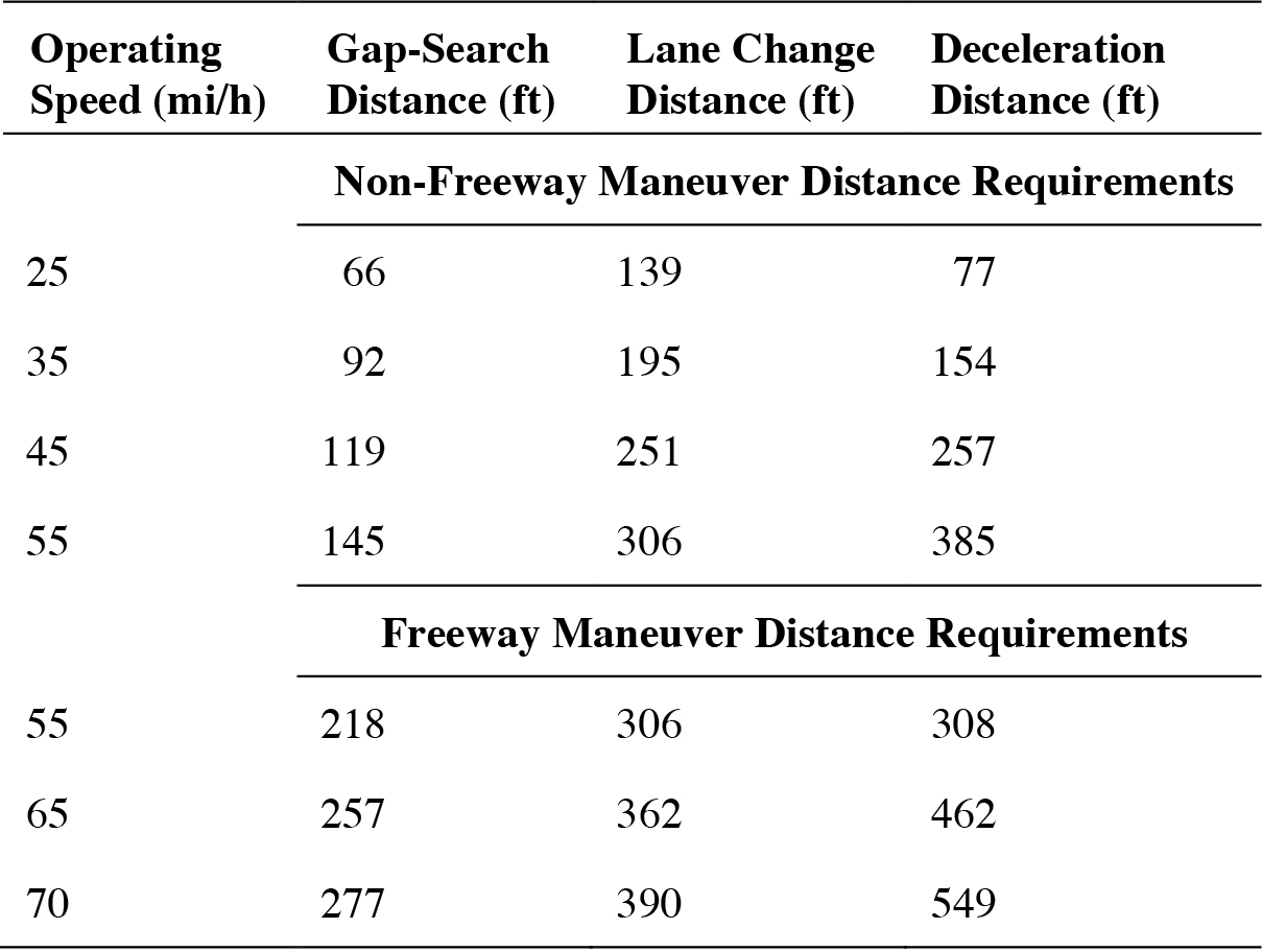
An example of required maneuver distances is provided in Table 27-8 for lane changes in preparation for a turn. These distances do not apply to situations in which drivers must stop. For high-volume roadways, more time may be needed to find a gap, while for low-volume roadways, some of the deceleration distance may overlap with the lane change distance.
Step 4. Calculate the Information Presentation Distance
The information presentation distance is the total distance from the choice point (e.g., intersection) at which the driver needs information. This distance is calculated using the following formula:

Long Description.
Information Presentation Distance equals Reading Distance plus Decision Distance plus Maneuver Distance
Source: Pline (2001)
Long Description.
The table has four column headings: Column 1: Operating Speed in miles per hour. Column 2: Gap-Search Distance in feet. Column 3: Lane Change Distance in feet. Column 4: Deceleration Distance in feet. The data for columns 2, 3, and 4 are grouped into two sections: Non-Freeway Maneuver Distance Requirements for rows 1 to 4 and Freeway Maneuver Distance Requirements for rows 5 to 7. The data for the Non-Freeway Maneuver Distance Requirements section are as follows: Row 1 Column 1: 25. Column 2: 66. Column 3:139. Column 4: 77 Row 2 Column 1: 35. Column 2: 92. Column 3: 195. Column 4:154 Row 3 Column 1:45. Column 2:119. Column 3: 251. Column 4:257 Row 4 Column 1: 55. Column 2: 145. Column 3: 306. Column 4: 385 The data for the Freeway Maneuver Distance Requirements section are as follows: Row 5 Column 1: 55. Column 2: 218. Column 3: 306. Column 4: 308 Row 6 Column 1: 65. Column 2: 257. Column 3: 362. Column 4: 462 Row 7 Column 1: 70. Column 2: 277. Column 3: 390. Column 4: 549
Step 5. Calculate the Legibility Distance
The legibility distance is the distance at which the sign must be legible. This distance is based upon the operating speed and the advance placement of the sign from the choice point. The legibility distance is calculated using the formula below:

Long Description.
Legibility Distance equals Information Presentation Distance minus Advance Placement
Step 6. Calculate the Minimum Letter Height
The minimum letter height is the height required for the letters on the sign based upon the legibility distance calculated above. It is also based upon the legibility index provided in the MUTCD (30 ft/in.).
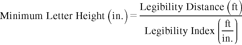
Long Description.
Minimum Letter Height open parenthesis in. close parenthesis equals start fraction Legibility Distance open parenthesis feet close parenthesis over Legibility Index open parenthesis feet over in. close parenthesis end fraction
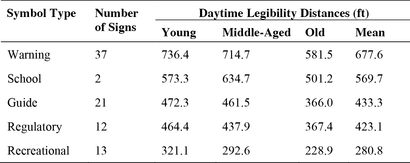
Another consideration is the minimum symbol size. The minimum symbol size is based upon the legibility distance of the specific symbol that is being used. Table 27-9 contains daytime legibility distances for five types of symbols based upon research (Dewar et al., 1994).
From these legibility distances, we can obtain two general trends: (1) legibility distances vary by sign type and (2) legibility distances are greatly reduced for older drivers. Legibility distances for symbols are generally greater than for word messages.
Example Application
As an example, a driver approaches an intersection on a 35-mi/h (51 ft/s) roadway. The driver needs to read a simple designation sign (D1-1) that contains one destination word and one symbolic arrow. The sign is placed 200 ft in advance of the intersection. The legibility index is assumed to be 30 ft/in. (FHWA, 2009). See Figure 27-9.
- Reading Distance (ft) = [(1 s/word)(1 word) + (0.5 s/symbol)(1 symbol)](51 ft/s) = 77 ft
- Decision Distance (ft) = (1 s/simple decision)(1 simple decision)(51 ft/s) = 51 ft
- Maneuver Distance (ft) = Gap Search (92 ft) + Lane Change (195 ft) + Deceleration (154 ft) = 441 ft
- Information Presentation Distance (ft) = Reading Distance (77 ft) + Decision Distance (51 ft) + Maneuver Distance (441 ft) = 569 ft
- Legibility Distance = Information Presentation Distance (569 ft) − Advance Placement (200 ft) = 369 ft
- Letter Height = (369 ft)/(30 ft/in.) = 12 in. (when rounded to the nearest inch)
Long Description.
The table has 3 primary column headings: Column 1: Symbol Type. Column 2: Number of Signs: Column 3: Daytime Legibility Distances in feet. Column 3 is subdivided into four sub columns: Column 3 a: Young Column 3 b: Middle Aged. Column 3 c Old. Column 3 d Mean. The data are as follows: Row 1 Column 1: Warning, Column 2: 37 Column 3 a:736.4 Column 3 b:714.7 Column 3c: 581.5 Column 3d: 677.6 Row 2 Column 1: School Column 2: 2 Column 3 a: 573.3 Column 3 b: 634.7 Column 3 c: 501.2 Column 3 d: 569.7 Row 3 Column 1: Guide Column 2: 21 Column 3 a: 472.3 Column 3 b: 461.5 Column 3 c: 366.0 Column 3 d: 433.3 Row 4 Column 1: Regulatory Column 2: 12 Column 3 a: 464.4 Column 3 b: 437.9 Column 3 c: 367.4 Column 3 d: 423.1 Row 5 Column 1: Recreational Column 2: 13 Column3 a: 321.1 Column 3 b: 292.6 Column 3 c: 228.9 Column 3 d: 280.8
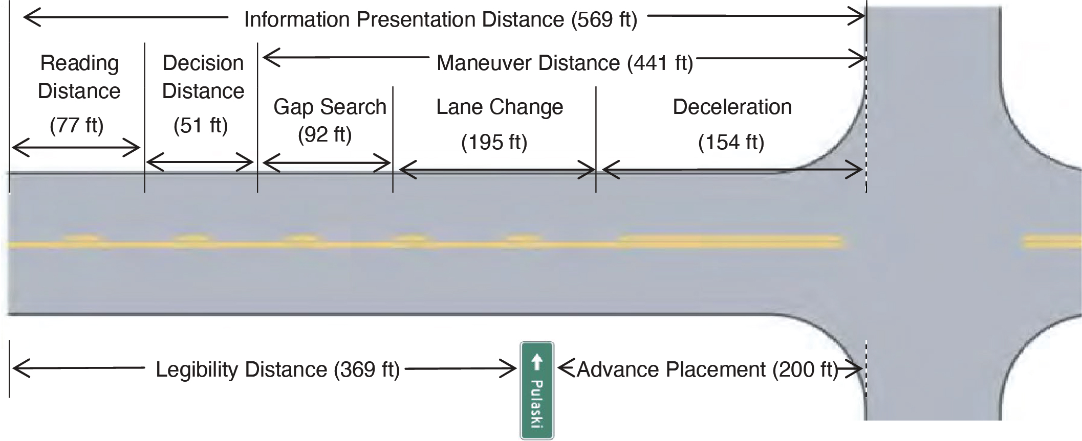
Long Description.
Line segments are marked above and below the road in the image. Above the road, entire distance of the road up to the intersection is marked by an information presentation distance segment, 569 feet. Below that is the Maneuver Distance segment, 441 feet which includes gap search, 92 feet, lane change, 195 feet, and deceleration, 154 feet, segments below. Prior to these segments are the reading distance, 77 feet, and decision distance, 51 feet, segments. Below the roadway a legibility distance segment, 369 feet, extends to a road sign for Pulaski. After the sign is the advance placement segment, 200 feet.
Tutorial 6: Calculating Appropriate CMS Message Length under Varying Conditions
The amount of information that can be displayed on a CMS is limited by the amount of time that the driver has to read the message. This amount of time, in turn, is determined by the legibility distance of the sign and the traveling speed of the passing vehicle. The legibility distance is the maximum distance at which a driver can first read a CMS message. According to Dudek (2004), this distance depends upon a number of factors, including:
- Lighting conditions
- Sun position
- Vertical curvature of the roadway
- Horizontal curvature of the roadway
- Spot obstructions
- Rain or fog
- Trucks in the traffic stream
These obstructions and visibility limitations reduce the amount of time that the sign is within view or legible, ultimately requiring a reduction in the amount of information that is displayed on the CMS. The information that can be displayed is measured in information units. An information unit is a measure of the amount of information presented in terms of facts used to make a decision. For example, the location of the problem, the audience that is affected by the problem, and the recommended action to take are each 1 information unit. To determine the appropriate number of information units for display on a CMS, the following steps should be considered.
Step 1. Determine the Legibility Distance for the CMS
The maximum legibility distance for a CMS depends on the design characteristics of the sign (Dudek, 2004). These characteristics include the display type, character height, character width, character stroke width, and the font displayed. The base legibility distances found in Table 27-10 are presented in Dudek (2004) and are based on the results of several studies. The distances are based on all uppercase letters, 18 in. character heights, approximately 13 in. character widths, and approximately 2.5 in. stroke widths. Note that all the information for light-emitting diode signs provided in this tutorial applies only to the newer aluminum indium gallium phosphide (or equivalent) LEDs.
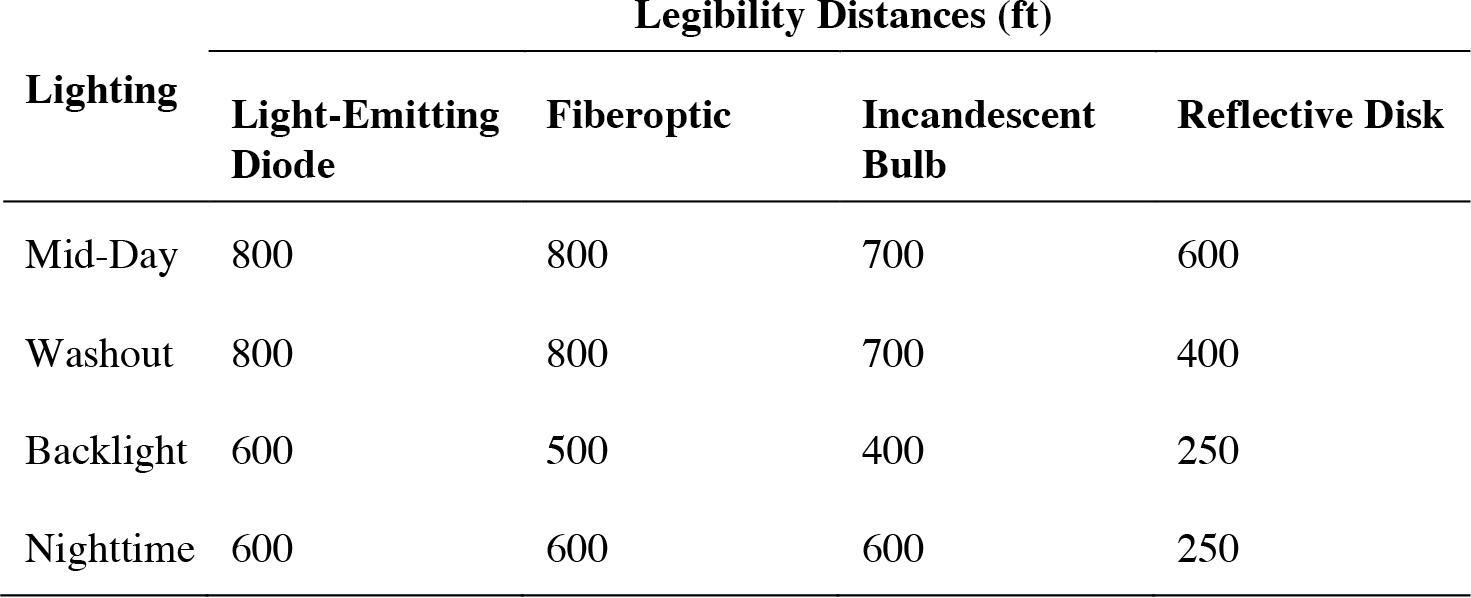
Source: Dudek (2004)
Long Description.
The table has 5 column headings. Column 1: Lighting. Column headings 2 to 5 are all legibility distances in feet for the following situations: Column 2: Light emitting diode. Column 3: Fiberoptic. Column 4: Incandescent Bulb. Column 5: Reflective Disk. The data are as follows: Row 1 Column 1: Mid Day Column 2: 800 Column 3: 800 Column 4: 700 Column 5: 600 Row 2 Column 1: Washout Column 2:800 Column 3: 800 700 Column 5: 400 Row 3 Column 1:Backlight Column 2:600 Column 3: 500 Column 4: 400 Column 5:250 Row 4 Column 1: Nighttime Column 2: 600 Column 3: 600 Column 4: 600 Column 5: 250
Step 2. Use the Driver Speed to Find the Base Maximum Number of Information Units Allowed in a Message
The maximum number of information units is derived from the legibility distance of the CMS (which depends on the technology used) and the speed of the passing vehicles. The faster the passing drivers are going, the less time they have to read the CMS message. Also, because the legibility distance of the sign depends upon the technology used, the number of information units also varies with the technology that is used. Finally, the diverse technologies perform differently under changing conditions. Table 27-11 presents the base maximum number of information units that can be presented for assorted CMS technologies, under several ambient lighting conditions.
Step 3. Adjust for Adverse Roadway and Environmental Conditions
There are many roadway and environmental conditions that reduce the visibility of CMSs and thus require a reduction in information units. Dudek (2004) provides further guidance on the exact number of information units that should be used under different conditions. The following sections describe how various conditions and factors lead to trade-offs in the number of information units that may be displayed.
Vertical Curves
The reduction in information units required for vertical curves depends on the design speed of the curve as well as the CMS offset from the road and the mounting height. The following general relationships apply to CMSs on vertical curves:
- As the design speed of the curve decreases, the number of information units that may be used decreases.
- As the horizontal offset from the road increases, the number of information units that may be used decreases.
- As the mounting height of the CMS decreases, the number of information units that may be used decreases.
In general, permanent CMSs that are mounted over the roadway are not affected by crest vertical curves (Dudek, 2004).
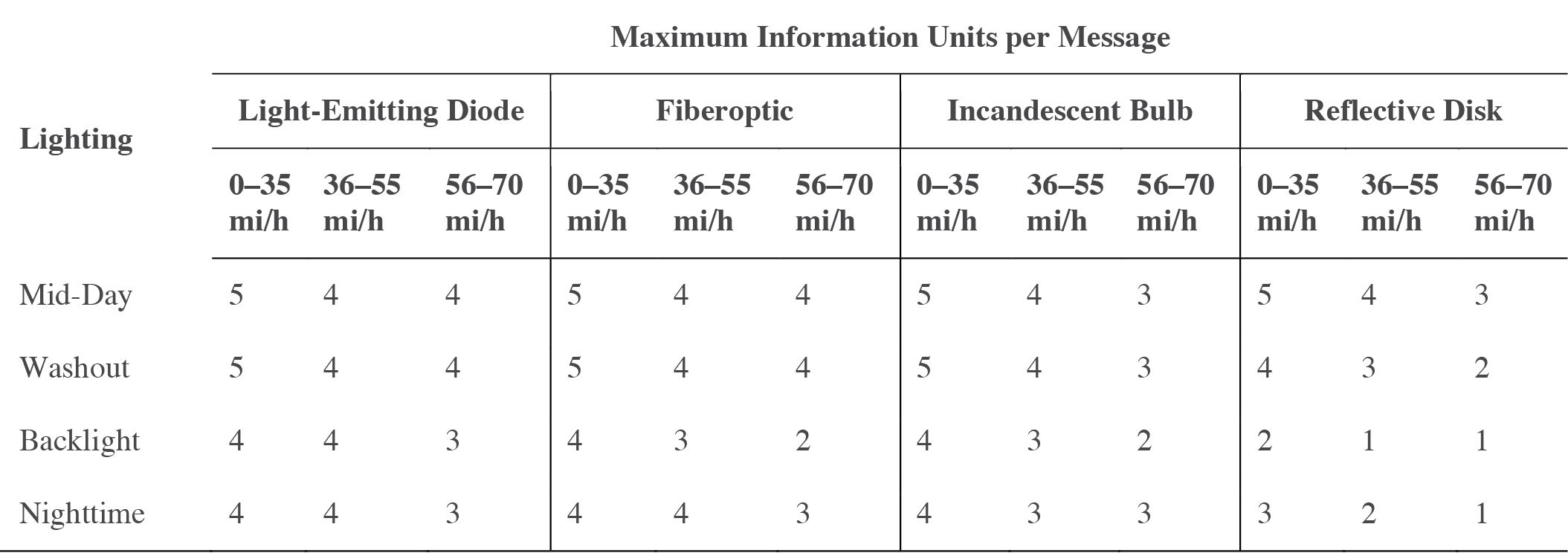
Source: Dudek (2004)
Long Description.
The table has 5 primary columns. Column 1: Lighting. Column 2: Light Emitting Diode. Column 2:Light-Emitting Diode. Column 3: Fiberoptic Column 4: Incandescent Bulb. Column 5: Reflective Disk. Columns 2 to 5 are each divided into 3 sub-columns: A: 0 to 35 miles per hour. B: 36 to 55 miles per hour. C: 56 to 70 miles per hour. Row 1 Column 1:Mid-Day Column 2 A: 5 Column 2 B: 4 Column 2 C: 4 Column 3 A: 5 Column 3 B: 4 Column 3 C: 4 Column 4 A: 5 Column 4 B: 4 Column 4 C: 3 Column 5 A: 5 Column 5 B: 4 Column 5 C: 3 Row 2 Column 1:Washout Column 2 A: 5 Column 2 B: 4 Column 2 C: 4 Column 3 A: 5 Column 3 B: 4 Column 3 C: 4 Column 4 A: 5 Column 4 B: 4 Column 4 C: 3 Column 5 A: 4 Column 5 B: 3 Column 5 C: 2 Row 3 Column 1:Backlight Column 2 A: 4 Column 2 B: 4 Column 2 C: 3 Column 3 A: 4 Column 3 B: 3 Column 3 C: 2 Column 4 A: 4 Column 4 B: 3 Column 4 C: 2 Column 5 A: 2 Column 5 B: 1 Column 5 C: 1 Row 4 Column 1: Nighttime Column 2 A: 4 Column 2 B: 4 Column 2 C: 3 Column 3 A: 4 Column 3 B: 4 Column 3 C: 3 Column 4 A: 4 Column 4 B: 3 Column 4 C: 3 Column 5 A: 3 Column 5 B: 2 Column 5 C: 1
Horizontal Curves
The main concern with CMSs located on horizontal curves is the obstruction of the sign by roadside objects. Permanent CMSs that are mounted above or adjacent to the travel lanes will likely be high enough to be seen over any roadside obstructions. However, portable CMSs are usually closer to the ground and more likely to be obscured by obstructions. In general, the number of information units that may be used decreases when:
- The obstruction gets closer to the roadway
- The curve radius decreases (i.e., for tighter curves)
Rain
Rain does not generally affect CMSs (Dudek, 2004). However, when the intensity of rainfall increases to 2 in./h or more, the visibility of the sign can be affected. When the operating speed of the roadway is over 55 mi/h, Dudek (2004) recommends that the number of information units displayed on portable LED CMSs should be reduced by 1 information unit. Portable LED CMSs often use fewer pixels per character and thus have lower luminance levels per character than permanent CMSs, which are relatively unaffected even in heavy rainfall. Therefore, signs utilizing other technologies should use fewer information units in heavy rainfall.
Fog
Fog can affect visibility even more than heavy rain. Generally, Dudek (2004) does not recommend a reduction in information units for permanent LED CMSs because of fog. A reduction is not necessary because of the high character luminance and contrast of permanent LED CMSs. However, portable LED CMSs require a reduction. The number of information units that may be used decreases when:
- The visibility range decreases
- The offset from the road increases
Trucks on the Roadway
Large trucks pose sight obstructions for other vehicles on the roadway. When a driverʼs view of a CMS is obscured by a truck, the driver has the option to change their speed or position to see around the truck. However, as the number of trucks on the roadway increases, the amount of space that is available for drivers to do this repositioning decreases. Thus, the more trucks that are on the roadway, the more likely they are to impair the view of a CMS for other drivers.
Step 4. Adjust for Blanking Time
Greenhouse (2007) found that inserting a 300-ms blank screen between phase 1 and phase 2 of a portable message sign improves comprehension. The study is further discussed in the “Displaying Messages with Dynamic Characteristics” guideline on page 22-10. Although the blanking time was only tested between phases 1 and 2 (not between 2 and 1), it is reasonably conceivable that drivers who see a blank between phases 1 and 2, but not between phases 2 and 1, would reverse the order of the phases and possibly have trouble understanding the message. Dudek (1992) recommends that blank time and/or asterisks should be displayed between cycles of a message that contains three or more phases (on one-word or one-line signs). Because one-word and one-line signs are more limited in the amount of information that they can display at one time, the phases may not make sense independently and drivers who read later phases before phase 1 may not understand the message. Thus, giving an indication of where the message is in the cycle gives drivers an idea of their location in the cycle.
Overall, drivers may use the blanking time to determine where they are in the message cycle, even before the message is legible to them. There are additional benefits in terms of message comprehension as shown by Greenhouse (2007). However, the insertion of blanking time reduces the total available time for the driver to read the message, potentially requiring a reduction in information units. Thus, there is a trade-off between the benefits of providing blanking time and the number of information units that may be contained in the message.
Step 5. Display the Resulting Number of Information Units
After the calculations and adjustments from Steps 1 through 4 are performed, the result will be the number of information units that may be displayed in the message. If there are still more information units in the message than should be displayed, they should be reduced using the following steps, until the appropriate number of information units is reached [steps and examples adapted from Dudek (2004)].
Step 5A: Omit and Combine Information Units
First, attempt to reduce the number of information units without losing content by following the steps below.
- Omit unimportant words and phrases
Example:
Original Message: |
Shortened Message: |
|||
ROAD CLOSED AHEAD |
ROAD CLOSED |
|||
DUE TO CONSTRUCTION |
1 MILE |
|||
FOLLOW DETOUR ROUTE |
FOLLOW DETOUR |
The word “Ahead” is unnecessary as drivers will assume the closure is ahead. The reason is less important than the location of the closure.
- Omit redundant information
Example:
Original Message: |
Shortened Message: |
|||
MAJOR ACCIDENT |
MAJOR ACCIDENT |
|||
ON I-276 NORTH |
PAST I-80 |
|||
PAST I-80 |
2 LEFT LANES |
|||
2 LEFT LANES CLOSED |
CLOSED |
If the CMS is on I-276, the same freeway as the accident, the information is evident to the drivers and may be omitted. The information units “2 Left Lanes Closed” and “Keep Right” are redundant because drivers can assume that if the two left lanes are closed, they will need to move to the right.
- Combine base CMS elements
Example:
Original Message: |
Shortened Message: |
|||
TRUCK ACCIDENT |
FREEWAY CLOSED |
|||
PAST I-80 |
EXIT AT I-80 |
|||
ALL LANES CLOSED |
FOLLOW DETOUR |
|||
AT I-80 |
||||
287 NORTH TRAFFIC |
In the previous example, the incident descriptor, incident location, and lanes closed message elements are combined into the information unit “Freeway Closed.” The location of the closure can be eliminated because the action element “Exit at I-80” describes the location.
Step 5B. Reduce the Number of Audiences in the Message
Example:
Original Message: |
Shortened Message: |
|||
I-76 CLOSED |
I-76 CLOSED |
|||
BEST ROUTE TO |
BEST ROUTE TO |
|||
PHILADELPHIA/I-95 |
PHILADELPHIA |
|||
USE RTE-73 NORTH |
USE RTE-73 NORTH |
When using this reduction technique, message designers must use their judgment to decide which audience is more important to address in the message. In the previous example, the audience “Philadelphia/I-95” was reduced from 2 information units to 1 information unit, “Philadelphia.”
Step 5C. Use Priority Reduction Principles
If the message still contains more information units than should be displayed, the information units should be reduced in order of priority. The priority order is derived from the information drivers need the most in order to make driving decisions. In Table 27-12, the information units are listed in priority order, with number 1 being the highest priority information.
If the closure is due to roadwork, the effect on travel and good reason for following the action should be eliminated. Even though the incident/roadwork descriptor is useful to drivers, it may be replaced with the lanes closed element if necessary. When choosing information units to eliminate, the designer should start deleting units from the bottom of these priority lists first (i.e., element numbers 8 or 6). More examples of the application of these steps can be found in Dudek (2004).
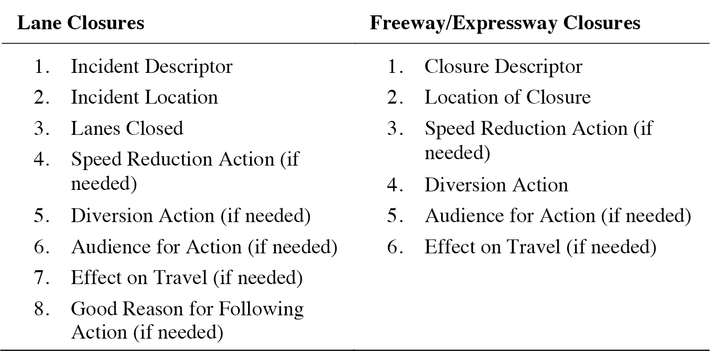
Long Description.
The order of priority for lane closures is as follows: 1. Incident Descriptor 2. Incident Location 3. Lanes Closed 4. Speed Reduction Action (if needed) 5. Diversion Action (if needed) 6. Audience for Action (if needed) 7. Effect on Travel (if needed) 8. Good Reason for Following Action (if needed). The order of priority for Freeway / Expressway closures is as follows: 1. Closure Descriptor 2. Location of Closure 3. Speed Reduction Action (if needed) 4. Diversion Action 5. Audience for Action (if needed) 6. Effect on Travel (if needed)
Tutorial 7: Joint Use of the Highway Safety Manual and the Human Factors Guidelines for Road Systems1
Background and Objectives
Using the Highway Safety Manual (HSM; AASHTO, 2010) and the Human Factors Guidelines for Road Systems (HFG) together provides a valuable resource for designing safer roadways. The HSM is used to quantify the effects of design and operational decision-making on crash frequency and severity outcomes, thus estimating the crash potential of roadway infrastructure alternatives. The HFG is used to facilitate operational decisions that reduce crash potential by providing currently accepted factual information and insight on road usersʼ needs. Together, these two documents enable highway planners, designers, operations engineers, and traffic engineers to incorporate features that promote the explicit consideration of crash potential for new or upgraded roadways.
Using the HSM and the HFG together enables highway planners, designers, operations engineers, and traffic engineers to better diagnose and address the contributing factors to crashes, thereby increasing the effectiveness of project treatment and selection. The joint use of the HSM and the HFG will improve end usersʼ ability to select roadway design and operational elements based on the best available data, thereby promoting an improved level of highway safety.
This tutorial summarizes a process that facilitates the combined use of the HSM and the HFG to support improved countermeasure selection for road safety. This tutorial is intended to be a short, instructive, and readily useful document that explains the joint use of these resources and provides state and local agencies a tool to enhance data-driven decision-making.
Overview of the HSM
The HSM was developed to provide tools and resources to help transportation practitioners make data-driven decisions to reduce crashes on all levels of roadways. Prior to the development of the HSM, there was no single resource to include crash potential in the project development and planning process. The use of the HSM has allowed for practitioners to not only include crash potential in decision-making but to utilize data as the cornerstone of those decisions.
The HSM is written for transportation professionals who:
- Have experience with the basic fundamentals of transportation safety,
- Are familiar with basic statistics and data interpretation, and
- Can exercise sound traffic safety and operational judgment.
The HSM provides guidance on traditional descriptive methods of analysis for traffic safety, while also driving the practice forward with predictive methods for crash analysis. When planning a new road or modifying an existing road, highway designers and traffic engineers must review and predict the expected safety of the new design. The methodologies presented in the HSM provide analytical tools for many types of roadway segments and intersections. The relative crash potential of design alternatives and traffic control can be reviewed and compared. The HSM focuses on quantifying safety performance within the domains of planning, design, operations, and maintenance, and is divided into four parts (see Figure 27-10).
In Volume 1, Part A, the user is provided with an introduction to the HSM and information about human factors and the fundamentals of highway safety performance.
Volume 1, Part B, covers the roadway safety management process. This part of the manual provides methods for network screening, crash diagnosis to understand potential contributing
_________________________
1This tutorial is adapted from Campbell, Hull, and Maistros (2018).
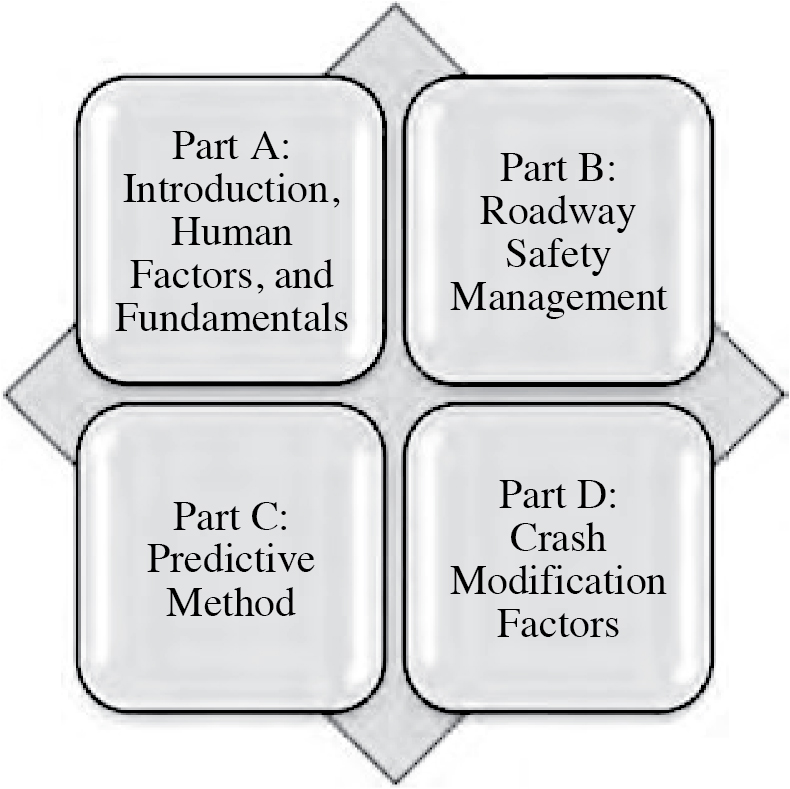
Long Description.
Part A: introduction, human factors and fundamentals; Part B: roadway safety management, Part C: predictive method, and Part D: crash modification factors.
factors and identifying treatments, and methods for selecting and prioritizing projects. These methods can be applied in near-term planning analysis, individual site evaluation, and the development of countermeasures.
In Volume 2, Part C, the predictive method is introduced for different facility types. The facility types are two-lane rural highways, multilane rural highways, and urban and suburban arterials. A Supplement, published in 2014, presents the predictive method for freeways, ramps, and ramp terminals. This project developed the predictive method for freeways and interchanges. The predictive method can be used to estimate the change in crash frequency or severity at a site as a function of traffic volume or roadway characteristics. These methods can be used in corridor-level alternatives analysis or more detailed site design.
Volume 3, Part D provides crash modification factors (CMFs) for use with Part B and existing facilities. Part D can only be used with Part B. Part C has its own CMFs for each facility type. CMFs are used to estimate the change in crash frequency that can be associated with a particular treatment.
CMFs can be used in the design exception process or site-specific evaluation process.
Together, the HSM and the HFG can supplement traditional sources of roadway design information and help improve decisions that reduce crash potential. They are both guidance documents intended to provide practitioners with practical information about quantitative crash reductions and human factors. There is valuable information in these documents that, when used in coordination, can reduce crash frequency and severity. Specifically, the HFG and HSM provide complementary information for finding countermeasures to design and operational factors leading to crashes.
A Process for Joint Use of the HSM and the HFG
In order to make the most effective and efficient use of the HSM and the HFG, a process comprised of the following five steps is recommended:
- Collect Site Data
- Review Site and Existing Conditions
- Identify Potential Countermeasures
- Develop and Prioritize Countermeasures
- Conduct Safety Effectiveness Evaluation
Each of the steps (the key five steps are in blue) is illustrated in Figure 27-11 and discussed in the following sections.
Step 1: Collect Site Data
Objective of Step 1: Compile data necessary to assess the traffic safety performance at the intended site quantitatively and qualitatively.
Data is the basis for defining how to improve traffic safety performance and understanding how to reduce the number and potential for crashes at a particular site. It is important to review recent projects that might impact crash potential (e.g., lane widening projects, horizontal curvature, or the installation of new sidewalks). The two critical types of quantitative data needed for this process are:
- Crashes.
- Traffic volumes.
These data types are subject to the following criteria: - Scale: Data may be presented at fine-grained individual levels or at more summary aggregate levels within a dataset. It is critical to understand the nature and scale of the data being used in the analysis process to ensure the appropriate measures are captured and addressed. As needed, describe and define scales and the units of measure associated with the data.
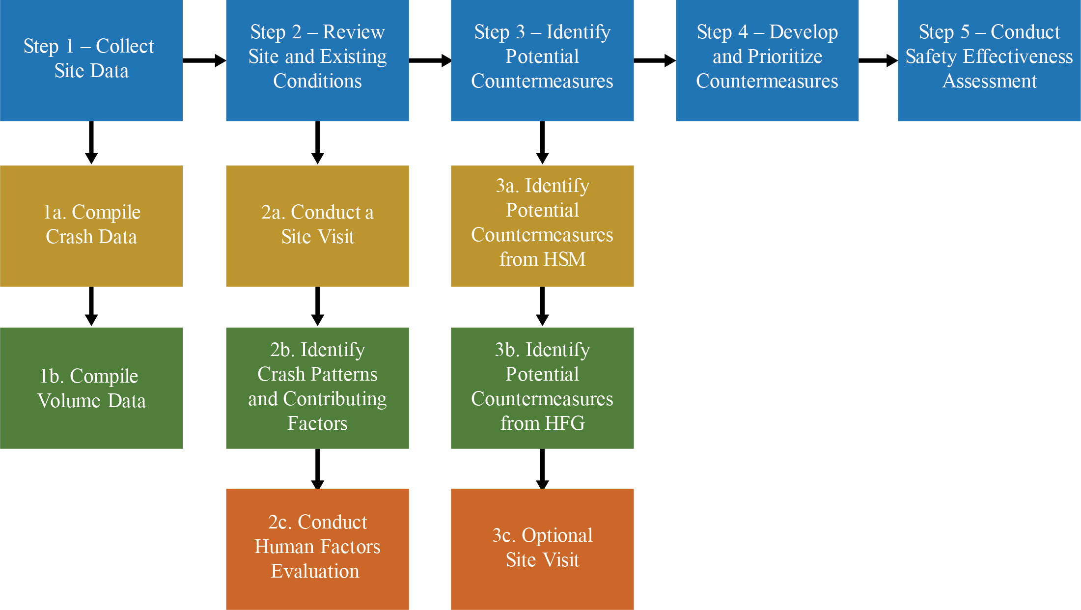
Long Description.
Step 1 – Collect Site Data 1a. Compile Crash Data 1b. Compile Volume Data Step 2 – Review Site and Existing Conditions 2a. Conduct a Site Visit 2b. Identify Crash Patterns and Contributing Factors 2c. Conduct Human Factors Evaluation Step 3 – Identify Potential Countermeasures 3a. Identify Potential Countermeasures from HSM 3b. Identify Potential Countermeasures from HFG 3c. Optional Site Visit Step 4 – Develop and Prioritize Countermeasures Step 5 – Conduct Safety Effectiveness Assessment
- Timeliness: It is important to understand the timeframe of each dataset used in this process. Because at least two quantitative data sources (crashes and traffic volumes) are being used (in addition to the consideration of recent projects that might impact crash potential), understanding when each data source was collected and the time periods it covers ensures that data comparisons are valid and that current issues are being addressed. Outdated information may lead to less accurate or effective results. One of the cornerstones of the HSM is the inclusion of crash rates, either in terms of crashes per year or crashes per traffic volume. These rates require multiple sources of information. Although it is not advisable to develop crash rates using crash data from 2015 and traffic data from 1997, the newest available data may vary by data type. For instance, crash data may be available for the most recent calendar year, while traffic data may lag a year behind. Some variances in timeliness are anticipated, but due diligence should be exercised to acquire the most recent available data.
- Quality/limitations: All data sets have known limitations or potentially even quality issues. Understanding where data is incomplete or known to have incorrect information is critical to successful analysis throughout this process.
The following data are typically obtained from a department of transportation (DOT), city, or metropolitan planning organization. Understanding which jurisdictions are responsible for the section of road being analyzed is important in determining the most valid source of crash/conflict data. There may be multiple sources of crash data for a particular facility if transportation departments and law enforcement maintain separate databases.
Step 1a. Compile Crash Data
- Scale: Crash data is commonly collected at three levels; crash, vehicle, person. Crash level data is the most summative and generally includes the information that describes the whole crash or facts applying to all parties involved in the crash (i.e., time, location, highest injury severity in a crash). Vehicle level data includes a record for each vehicle involved in the crash, and person level data includes a record for each individual involved in the crash.
- Timeliness: A minimum of five years of crash data is recommended for analysis. While electronic crash reporting has greatly reduced the processing time for crashes, it is still common to have delays of a year or more. As such, the most recent crash data may not cover the most recent calendar year.
- Quality/limitations: Each crash database has its own intricacies and limitations. Take time to either read the metadata associated with the crash data, or to talk with the crash data managers to understand the limitations or known quality issues.
In some situations, crash data availability may be limited. The HSM and HFG are both based on data and address safety issues identified through data analysis. Efforts should be made to capture available safety data; however, there are options for conducting analyses without data. The HSM, specifically, can estimate the number of crashes at a site with safety performance functions (SPFs). These estimations can then be adjusted with potential improvements/changes to estimate crash potential. While these processes have the flexibility to estimate safety benefits without crash data, the results are much more reliable and reflect the specific project location characteristics.
Step 1b. Compile Volume Data
- Scale: Volume data is needed for each transportation mode in the analysis scope. Certain modal volumes, such as those for bicycles and pedestrians, are often difficult to obtain. Guidance for obtaining these volumes can be found in NCHRP Report 770: Estimating Bicycling and Walking for Planning and Project Development (Kuzmyak et al., 2014). An additional source is Washington DOTʼs Methods for Estimating Bicycling and Walking in Washington State (Nordback
- and Sellinger, 2014). It is also critical to use volume data with enough information to distinguish important traffic patterns. For example, if an intersection with two-way stop control is being evaluated, it is important to know not just the total volume for the intersection but the major versus minor road traffic and any turning traffic as well.
- Timeliness: The most recent volume data available should be used. If there was a major change in traffic during the crash analysis period, it may be prudent to use volume data reflecting this change for the appropriate years.
- Quality/limitations: As with scale, it is important to understand which modes and traffic patterns the volume data pertains to. Any quality issues or known limitations of the crash/conflict data should be described. Patterns of crashes may also appear in the volume data. For example, if 50 percent of the crashes occur during the peak hours 7 a.m. to 9 a.m. turning left northbound, then a field investigation should be conducted during that timeframe.
Roadway facilities are subject to a wide variety of revision projects, from lane widening, changes in horizontal curvature, and the installation of sidewalks to new mailboxes and signs. The scale, timeliness, and known limitations in the type, amount, or quality of the data associated with these projects should be considered. Projects occurring within the data analysis period need to be considered for their impact on traffic patterns and safety performance. If major projects occurred just before the crash data period being analyzed, it may be prudent to expand the crash data period, if possible. Data and project plans are not necessarily data available for all projects at a site. For example, smaller projects such as signs, post boxes, or other installations may not require project plans but may affect sight lines or clear zones.
Anticipated Outcome of Step 1
A time-consistent collection of crash, traffic, and project data describing the safety, behavioral, and roadway data relevant to the site.
Step 2: Review Site Conditions
Step 2a. Conduct a Site Visit
Objective of Step 2a: Conduct a qualitative analysis of existing roadway, behavioral, and human factors conditions at the site.
Visit the site under daytime and nighttime conditions, during the peak and off-peak hours. (If a site visit is not possible, a videolog or online street mapping tool could be used.) Visiting the site at a variety of times is helpful for understanding the conditions facing road users (or virtual road users, if new plans or designs are being evaluated at the site) under a variety of circumstances. The purpose of these visits is to determine the conditions facing road users and potentially affecting traffic safety. Conditions may include infrastructure, behavioral, and operational factors.
- Infrastructure: Focus on the built environment at the site. What is the state of the infrastructure that road users are dealing with? Items to consider include:
- pavement and sidewalk condition,
- sign and marking visibility,
- drainage issues, shoulder condition,
- vegetation maintenance,
- the proper functioning of signals (including pedestrian signals),
-
- roadway and intersection lighting, and
- any differences in upstream geometric or traffic control conditions that may impact user decisions.
- Behavioral and Human Factors: How are road users responding to the built environment and traffic within and upstream of the project? Items to consider include:
- driversʼ use of passing or turning lanes,
- line-of-sight issues (to both signal and other traffic control devices),
- bicyclists or pedestrians traveling along shoulders, and
- pedestrian mid-block crossings.
- Operational: How can drivers be better directed and informed to move more efficiently and with less potential for a crash? Items to consider include:
- large queues from turning traffic,
- traffic frequently blocking intersections,
- signal timing, non-conforming signing and marking, and
- cues that might lead to road user indecision, among others.
These site visits are similar to road safety audits (RSAs) and may be conducted as informal RSAs. An RSA is a formal safety performance examination of an existing or future road or intersection by an independent, multidisciplinary team. These assessments usually offer a qualitative approach to understanding safety and potential alternatives but do not always provide the quantitative approach of this HSM/HFG process. Although a formal RSA may not be completed, several guiding prompt sheets have been developed for RSAs that can be useful during a site visit. Figure 27-12 provides an example prompt sheet for existing roadways. Several prompt sheets for specific audits are available from the FHWA at https://safety.fhwa.dot.gov/rsa/.
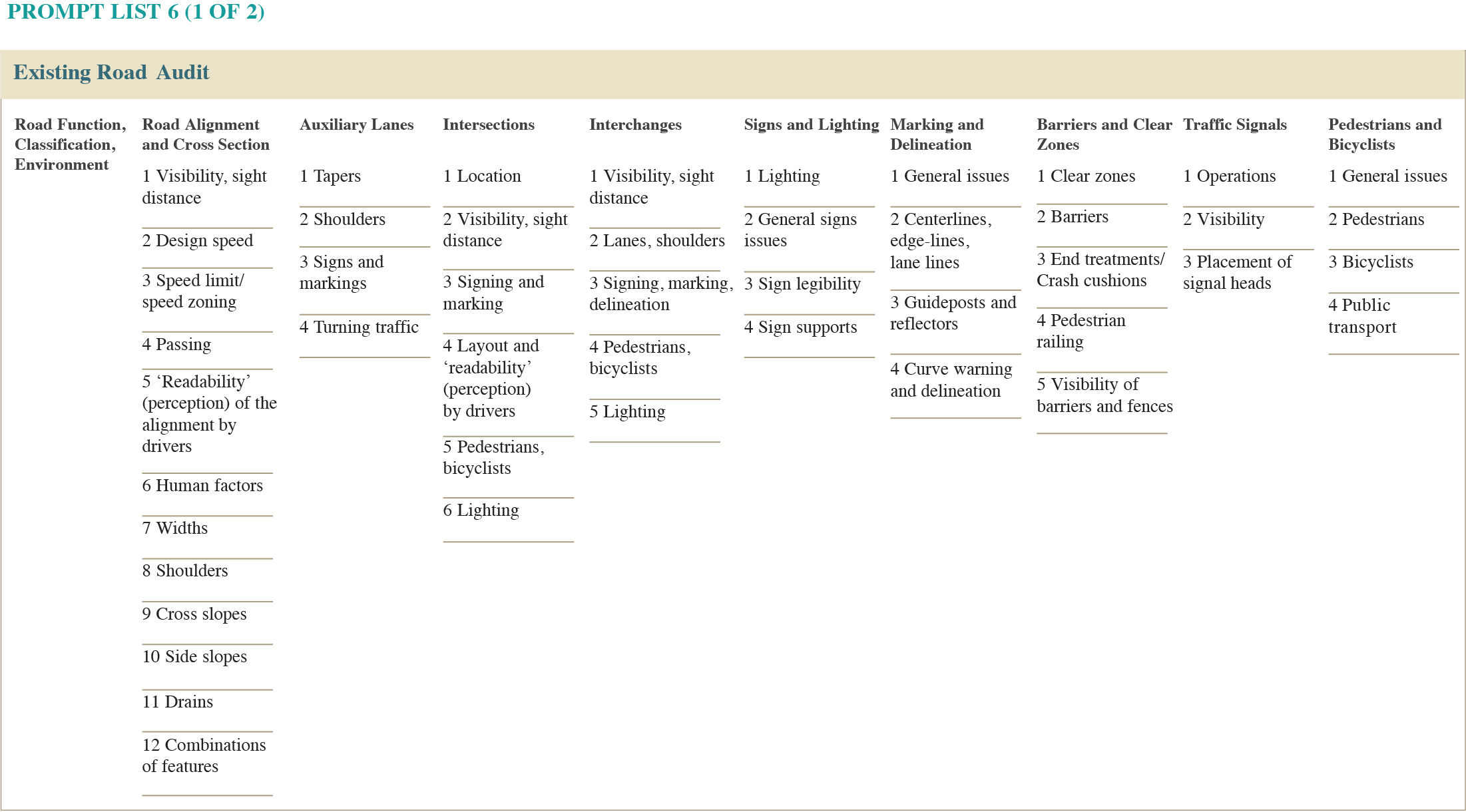
Source: Ward (2006)
Long Description.
There are 9 column headers that are all labeled as Road functions, classifications and environment. The column headers are: road alignment and cross section; auxiliary lanes; intersections; interchanges; signs and lighting; marking and delineation; Barriers and clear zones; Traffic signals; and pedestrians and bicyclists. The column for road alignment and cross section has 1 Visibility, sight distance 2 Design speed 3 Speed limit/speed zoning 4 Passing 5 ‘Readability’ (perception) of the alignment by drivers 6 Human factors 7 Widths 8 Shoulders 9 Cross slopes 10 Side slopes 11 Drains 12 Combinations of features. The column for Auxiliary Lanes has 1 Tapers 2 Shoulders 3 Signs and markings 4 Turning traffic The column for Intersections has 1 Location 2 Visibility, sight distance 3 Signing and marking 4 Layout and ‘readability’ (perception) by drivers 5 Pedestrians, bicyclists 6 Lighting The column for Interchanges has 1 Visibility, sight distance 2 Lanes, shoulders 3 Signing, marking, delineation 4 Pedestrians, bicyclists 5 Lighting The column for Marking and Delineation has 1 General issues 2 Centerlines, edgelines, lane lines 3 Guideposts and reflectors 4 Curve warning and Delineation The column for Barriers and Clear Zones has 1 Clear zones 2 Barriers 3 End treatments /Crash cushions 4 Pedestrian railing 5 Visibility of barriers and fences The column for Traffic Signals has 1 Operations 2 Visibility 3 Placement of signal Heads The column for Pedestrians and Bicyclists has 1 General issues 2 Pedestrians 3 Bicyclists 4 Public transport
Anticipated Outcome of Step 2a
A qualitative analysis of traffic, behavioral, and roadway issues at the site.
Step 2b. Identify Crash Patterns and Contributing Factors
Objective of Step 2b: To quantitatively describe the safety performance at the site by mode, year, crash type, and contributing factor. Crash examples are illustrated but if such data are not available, conflict statistics, such as police reports/citations, can be substituted for crashes.
Understanding crash trends for the site is crucial for quantitatively assessing the siteʼs potential for crash reduction. There are several ways to effectively summarize crash trends, and no single set of tables or charts is universally correct. While the quantity, format, and style of the trends are up to the developer, it is important to clearly and completely describe the crash statistics by mode, year, and severity. As noted in Step 1, it is also important to use the number of crashes and the count of injuries for the crash trend analysis. Figures 27-13, 27-14, and 27-15 illustrate the data breakdowns that should be included in the crash summary; additional tables or graphs may be included as needed.
Develop a Statement of Significant Trends and Findings
Based on the totality of the crash/conflict record, a short summary of significant trends or findings should be developed. The state of significant trends and key findings should focus on the more severe crashes and look for crash types and contributing factors where the severe crashes are over-represented. For example, in Figure 27-14, the crash type with the greatest number of crashes was rear-end, however, all of the crashes were non-injury, PDO crashes. Conversely, all ten of the ‘Vehicle hit pedestrian’ crashes were either fatal, serious, or evident-injury crashes. The number of pedestrian crashes would be a significant finding that would warrant identification and perhaps some brief discussion. Note in Figures 27-13, 27-14, and 27-15 how the manner in which the total number of crashes is presented in each of the tables is different, but that all of the figures are equally important and are needed to illustrate the breadth of the potential contributing factors and crash types.
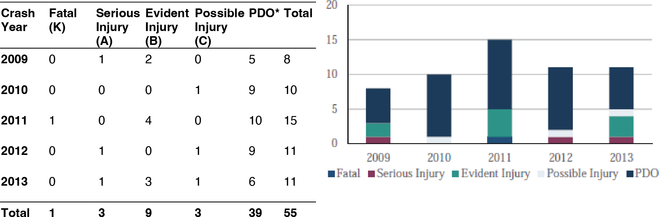
*Property damage only
Long Description.
The table has six columns and seven rows. The column headers are Fatal (K), Serious injury (A), Evident injury (B), Possible injury (C), PDO, and Total. The row headers are Crash Year, 2009, 2010, 2011, 2012, 2013, and Total. The data for the first row are 0, 1, 2, 0, 5, 8. The data for the second row are 0, 0, 0, 1, 9, 10. The data for the third row are 1, 0, 4, 0, 10, 15. The data for the fourth row are 0, 1, 0, 1, 9, 11. The data for the fifth row are 0, 1, 3, 1, 6, 11. The data for the final row are 1,1 3, 9, 3, 39, 55. A note explains that PDO means property damage only. The vertical stacked bar graph plots numbers from 0 to 20 on the vertical axis in increments of 5 and years from 2009 to 2013 on the horizontal axis. The bars represent fatal, serious injury, evident injury, possible injury, and PDO.
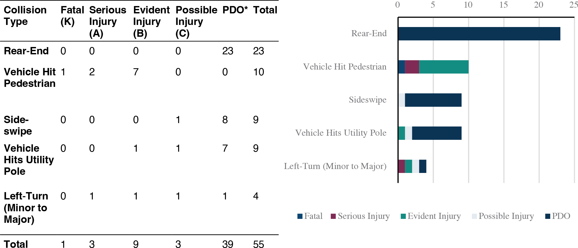
*Property damage only
Long Description.
Each row in the table shows data for a collision type. The column headers are Fatal (K), Serious Injury (A), Evident Injury (B), Possible Injury (C), PDO, and Total. The data for each collision type row are as follows: Rear-End 0, 0, 0, 0, 23, 23. Vehicle Hit Pedestrian 1, 2, 7, 0, 0, 10. Side-swipe 0, 0, 0, 1, 8, 9. Vehicle Hits Utility Pole 0, 0, 1, 1, 7, 9. Left-Turn (Minor to Major) 0, 1, 1, 1, 1, 4. Total 1, 3, 9, 3, 39, 55. A note explains that PDO means property damage only. The stacked horizontal bar graph plots the numbers from 0 to 25 on the horizontal axis in increments of 5. The vertical axis shows rear-end, vehicle hit pedestrian, sideswipe, vehicle hits utility pole, left-turn (minor to major). The bars represent fatal, serious injury, evident injury, possible injury, and PDO.
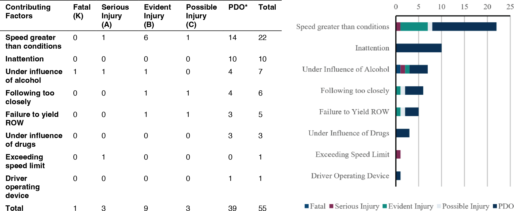
*Property damage only
Long Description.
Each row in the table shows data for a contributing factor. The column headers are Fatal (K), Serious Injury (A), Evident Injury (B), Possible Injury (C), PDO, and Total. The data for each contributing factor row are as follows: Speed greater than conditions 0, 1, 6, 1, 14, 22. Inattention 0, 0, 0, 0, 10, 10. Under influence of alcohol 1, 1, 1, 0, 4, 7. Following too closely 0, 0, 1, 1, 4, 6. Failure to yield ROW 0, 0, 1, 1, 3, 5. Under influence of drugs 0, 0, 0, 0, 3, 3. Exceeding speed limit 0, 1, 0, 0, 0, 1. Driver operating device 0, 0, 0, 0, 1, 1. Total 1, 3, 9, 3, 39, 55. The stacked horizontal bar graph plots the numbers from 0 to 25 in increments of 5 on the horizontal axis. The vertical axis shows speed greater than conditions, inattention, under influence of alcohol, following too closely, failure to yield ROW, under influence of drugs, exceeding speed limit, and driver operating device. The bars represent fatal, serious injury, evident injury, possible injury, and PDO.
Anticipated Outcome of Step 2b
A quantitative description of the safety challenges at the site with an understanding of the critical crash types, severities, and contributing factors
Step 2c. Conduct Human Factors Evaluation
Objective of Step 2c: Review crash or conflict data summaries and the site visit results to identify possible human factors issues for consideration in developing robust, science-based safety countermeasures.
Below, we provide a brief overview of the human factors approach to road safety, followed by a set of specific steps needed to conduct a human factors evaluation of existing conditions at an existing site.
Overview of the Human Factors Approach to Road Safety
A human factors evaluation of a specific roadway site starts with an understanding of the human factors approach to driving and road safety performance. At its core, this approach considers and accounts for road user needs, capabilities, and limitations in: (1) the design and operation of roads, vehicles, and pedestrian/bicycle/transit facilities, and (2) the identification of causal factors underlying conflicts and crashes. Figure 27-16 illustrates how the road user, vehicle, and the roadway environment intersect and interact during the driving task to support safety.
The “road user” factor includes capabilities and limitations such as age, training, experience, road familiarity, and possible impairment; the “environment” factor includes elements like road geometry, traffic control devices, and the luminance levels of signs and markings; and the “vehicle” factor includes automobile and truck components like tires, brakes, or special safety systems.
Safety performance reflects how well these components interact and work together to support full and accurate extraction of information and understanding of environmental cues and emerging situations that lead to effective decision-making by road users. Specifically:
- The road user
- samples information from the environment,
- controls vehicles, bicycles, or walks through a facility, and
- maneuvers through the environment.
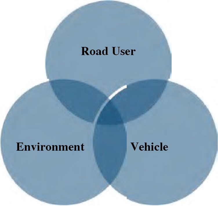
- The environment
- provides information to the road user,
- helps develop and support user expectations, and
- responds to the road user (e.g., a driver) through actions of other road users.
- The vehicle
- triggers some responses in the environment,
- serves as a stimulus to other road users (e.g., pedestrians and bicyclists pay close attention to nearby vehicles), and
- provides feedback to all road users (driver, pedestrians, bicyclists).
A useful way to think about how road users, particularly drivers, interact with the road environment is to examine typical visual scanning behaviors and patterns. Figure 27-17 illustrates such visual scanning behaviors; a key element is that road users are continually seeking to extract the most meaningful information (MMI) from the roadway scene by scanning segments of the roadway in iterative steps. The sampling frequency will vary and can be influenced by factors such as the road user, type of operation, roadway type, and environmental conditions. In this context, the specific MMI for a specific user at a given roadway location will also vary and could range from roadway edges or markings to signs or traffic control devices to objects moving within the scene, such as pedestrians or bikes.
Critically, it is often the interactions between road users, vehicles, and the environment that lead to errors, conflicts, crashes, and fatalities. Specifically, errors do not generally reflect a problem with a single factor—as in models of crashes that refer to a broken link in a causal chain—but, rather, reflect a confluence of factors that occur more or less simultaneously. For example, a crash doesnʼt generally happen just because a driver is older; rather, it might happen to an older driver who was driving at night, under bad weather conditions, and faced a sign that was wordy, complicated, damaged, or worn out. As illustrated in Figure 27-18, this view of crashes is well-supported by crash data (Treat et al., 1979). The figure shows that while drivers contributed to 93 percent of crashes, they were the sole cause of only 57 percent of these crashes. The crash percentages in the shaded regions of the figure highlight the role of driver, roadway, and vehicle interactions as causal factors in crashes.
Consider some other examples with multiple factors:
- On a wet road, worn brakes or tires lead to increased stopping distances and an increased probability of a rear-end crash.
- No lighting and dark clothing with or without a pedestrian crosswalk increasing the probability of a pedestrian crash in nighttime conditions.
- Drivers impaired by distraction, drugs, or alcohol; who are more easily confused by complex geometrics, signing; and who have an increased probability of a crash.
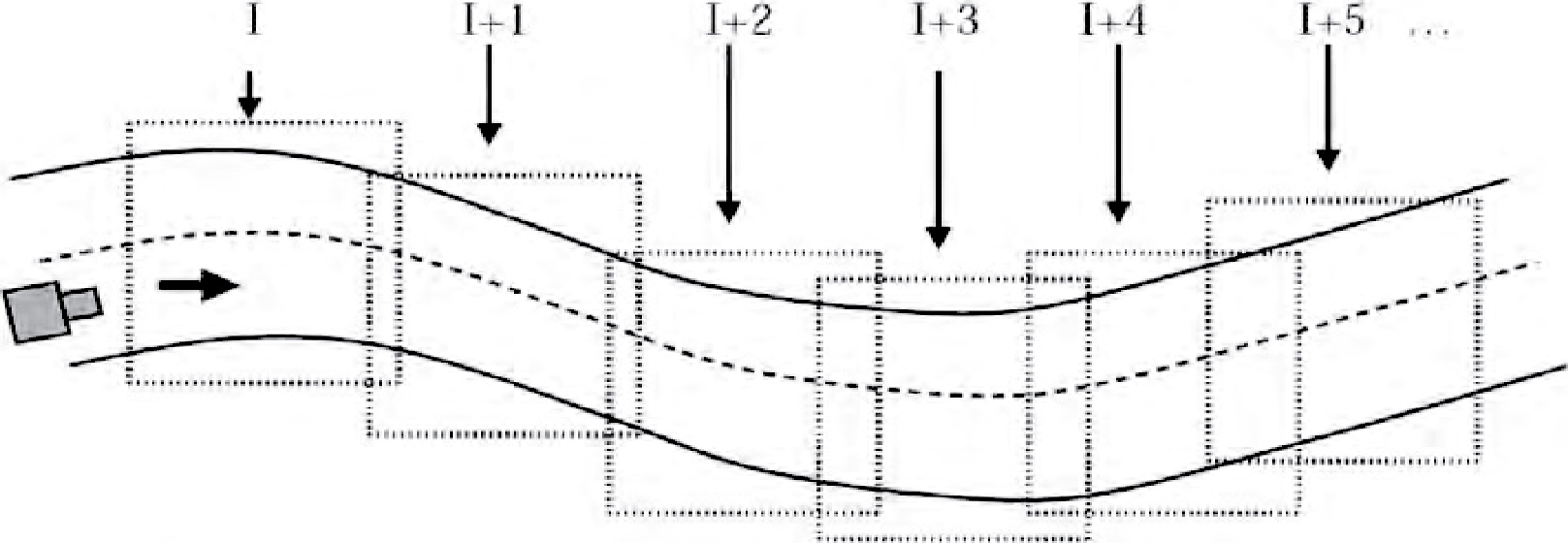
I = User scanning steps (vary in size)
Long Description.
Arrows point from I, I plus 1, I plus 2, I plus 3, I plus 4, and I plus 5 to different points on the road. I is user scanning steps (vary in size).
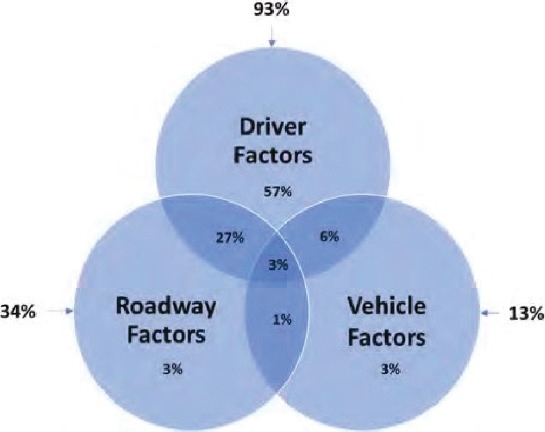
Source: Treat et al. (1979)
Long Description.
The circles represent 34 percent roadway factors, 13 percent vehicle factors, and 93 percent driver factors.
The critical takeaway here is to consider the full range of contributing factors that interact with a specific context and eventually lead to errors and crashes.
Develop the Human Factors Interaction Matrix. The Haddon Matrix was developed by William Haddon (see Haddon 1964, 1972, and 1980) to improve emergency responses for people injured in crashes and provides a technique for examining factors related to attributes of individuals, vehicles, and the environment before, during and after a crash that results in injury or death (see also Table 6-1 from the HSM). The goal for the HFG/HSM user is similar, i.e., to consider and list the individual road user, vehicle, and environmental factors (and any potential interactions) that could contribute to driver confusion, misperceptions, high workload, distraction, or other problems and errors.
Under the HFG framework, a modified Haddon Matrix called the Human Factors Interaction Matrix (HFIM) is used to help identify factors related to the road user, vehicle, and the environment, as well as interactions between these factors that could contribute to a reduction in road safety across various scenarios and driving situations. Table 27-13 shows a blank HFIM.
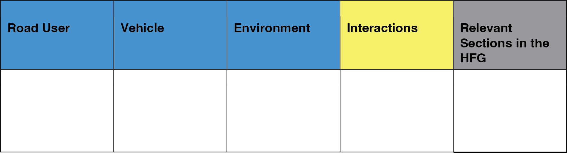
Long Description.
The column headings for the HFIM table are as follows: Column 1: Road User. Column 2: Vehicle. Column 3: Environment. Column 4: Interactions. Column 5: Relevant Sections in the HFG.
From the left, the first four columns of this table are to be filled out as part of Step 2: “Review Site Conditions” in the “joint use” process. The last column, “Relevant Sections in the HFG,” will be filled out later as part of Step 3: “Identify Potential Countermeasures.” The HFIM is typically a one-way table organized by columns. Note that the information in the HFIM is organized by columns, not rows, and that adjacent information (information to the left or right) is not necessarily related.
A version of the HFIM is shown in Table 27-14 and it is filled-in with a set of factors as examples that could contribute to reductions in roadway safety. Note that this is not a comprehensive set of factors, but only a list of possible factors that could apply to a range of crash scenarios. Filling out this table requires thinking about and listing the individual road user, vehicle, and environmental factors (and any possible interactions) that could contribute to reductions in road safety performance.
When completing the HFIM, users should recognize that the individual elements and their interactions need to reflect the specific type of vehicles and types of road users using the infrastructure. For example, you can have large semi-trucks on some roads but not on others; e.g., some bridges and parkways. Also, you cannot have pedestrians on interstates (except in emergency). Certain situations, such as work zones, require special consideration of the locations of maintenance staff and temporary signage. While the focus of the table should be on potential contributors to errors and crashes, the table could also include positive elements; i.e., compensatory features of the site that could mitigate the factors that are potentially contributing to crashes. Overall, the factors included in the HFIM should reflect careful consideration of the situation at hand, the crash record, and all possible impacts on the safety performance of the facility.
Finally, keep in mind that solutions (in the form of countermeasures or treatments) are not being sought at this stage. The focus here is on identifying and understanding those roadway components that could be contributing to driver confusion, misperceptions, high workload, distraction, or other potential driving errors at a particular site.
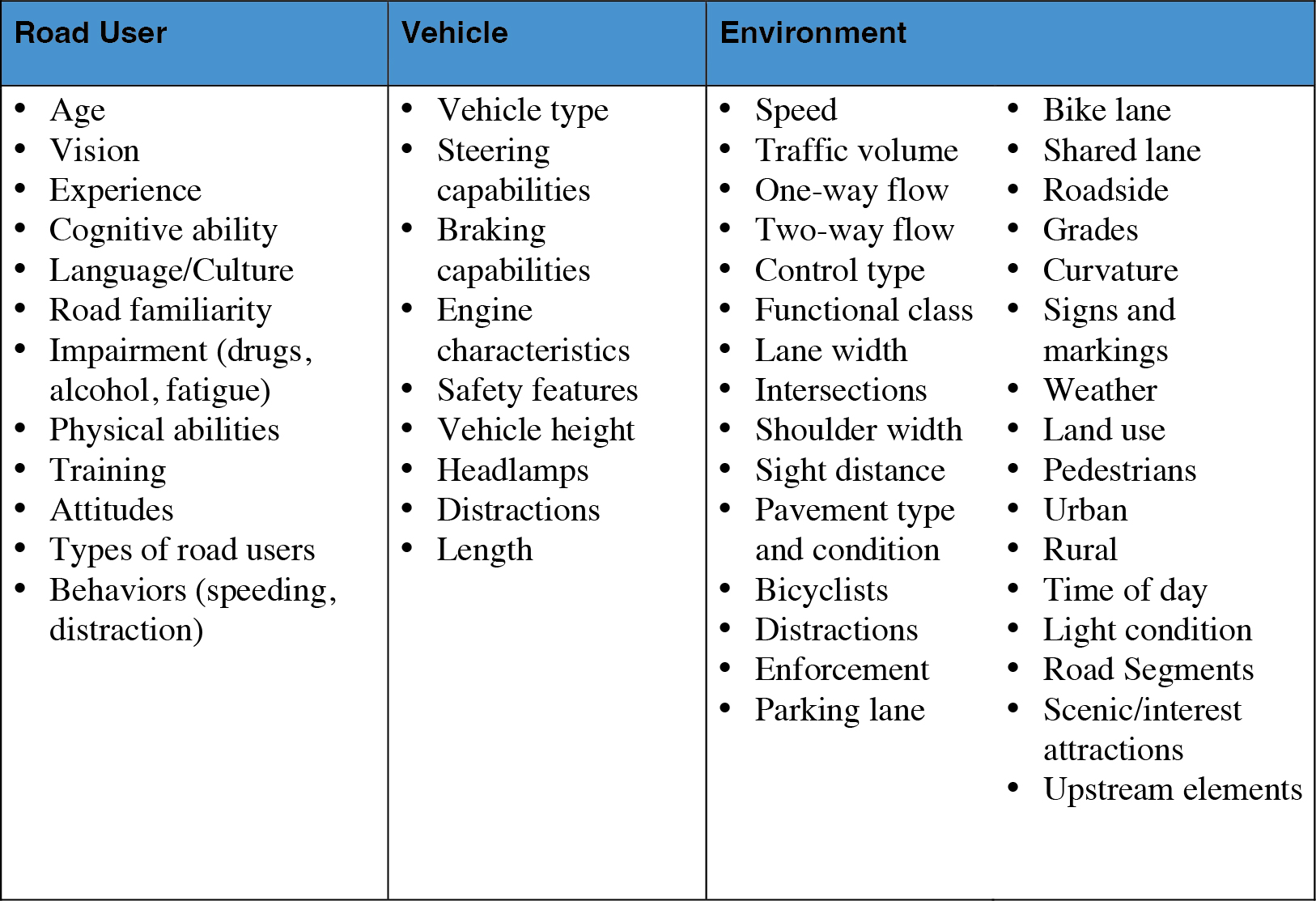
Long Description.
The road user factors listed are as follows: Age; Vision; Experience; Cognitive ability; Language/Culture; Road familiarity; Impairment (drugs, alcohol, fatigue); Physical abilities; Training; Attitudes; Types of road users; Behaviors (speeding, distraction). The Vehicle factors are as follows: Vehicle type; Steering capabilities; Braking capabilities; Engine characteristics; Safety features; Vehicle height; Headlamps; Distractions; Length. The Environment factors are as follows: Speed; Traffic volume; One-way flow; Two-way flow; Control type; Functional class; Lane width; Intersections; Shoulder width; Sight distance; Pavement type and condition; Bicyclists; Distractions; Enforcement; Parking lane Bike lane ; Shared lane; Roadside; Grades; Curvature; Signs and markings; Weather; Land use; Pedestrians; Urban; Rural; Time of day; Light condition; Road Segments; Scenic/interest attractions; Upstream elements.
In filling out an HFIM table, the objective is to consider and document the possible road user, vehicle, and environment issues that could contribute to confusion, errors, and crashes at the site or traffic situation that you are evaluating. Key inputs to the process of completing an HFIM table include:
- The basic crash or conflict data compiled in Step 1,
- The site visit results from Step 2a (including relevant site data such as the types of vehicles, cross-section dimensions, traffic volumes, speed limits, kinds of traffic control),
- Considerations of infrastructure elements upstream of individual crash sites, and
- The crash data summaries from Step 2b.
At this early stage in the process, it is best to generate an HFIM table that includes all possible factors impacting safety performance rather than generating a more selective list. Specifically, the HFIM should include any factors and combinations of factors (interactions) that could reasonably contribute to the known or suspected opportunities for reducing crash potentials at the site under investigation. Broad considerations should include:
- The type, frequency, and severity of the crash or conflict,
- Contributing factors, and
- On-the-scene observations of the facility and representative traffic movements (including pedestrians, bicyclists, and transit vehicles).
In this regard, some interactions may be quantitative and very specific, while others may be qualitative and reflect possible effects.
As noted earlier, most crashes (or conflicts and near-misses) are the results of interactions among two or more of the individual factors listed in the HFIM. Therefore, identifying known or possible crash- or conflict-relevant interactions will be critical to identifying potential countermeasures in Step 3. Carefully think as a virtual user through ways in which the individual factors could—in combination—create confusion, distraction, uncertainties, or misperceptions. Document those factors that are likely to have these effects in driving scenarios and road user behaviors, especially considering the site-specific crash and safety data.
Some specific questions to ask include the following:
- What is the nature of the observed crashes/conflicts? Are there any discernible patterns between or among PDO crashes/conflicts and crashes/conflicts involving serious injuries or fatal crashes?
- What can the most common crash types (e.g., rear-end crashes or “vehicle hit pedestrian”) tell us about the relative contribution of road user, vehicle, and environment issues to the crashes?
- What are the most common contributing factors cited in the crash records?
- From the perspective of a road user (both the typical road user as well as a road user who may be older or impaired in some way), what might be some sources of confusion when trying to extract the MMI from the road geometry and traffic control information? In general, is there consistency and meaning to the geometrics, signs, markings, and traffic control devices that road users rely on?
- How might unique issues associated with vehicle type be contributing to crashes or conflicts? For example, does vehicle size play a role in how well the driver or road user can see signs, markings, and other road users, or how well the driver can navigate through a roadway with narrow lanes and no shoulders?
- Are there any unique environmental and road conditions that substantially increase road user stress, comprehension time for roadway information, or response maneuvers to hazards at conflict points? Examples may include short acceleration/deceleration lanes, unexpected roadside hardware placement, unexpected narrowed lane widths, significant visibility restrictions, steep grades, and other similar conditions.
- In general, are there any unclear or misleading cues between the roadway and user? Such cues may be the lack of a timely (or conflicting) presentation of geometric, signing or pavement marking information. Examples are: using non-standard or non-maintained lanes or shoulders, less that standard sight distance for conditions, less than standard distance for acceleration or deceleration of vehicle, or where the speed differential is more than 15 mph.
Consider not just the factors that were present at the exact time of a crash but also factors or events that could have occurred prior to the crash.
Anticipated Outcome of Step 2c
A HFIM that is populated with possible road user, vehicle, and environment issues – and their interactions – that could be impacting the safety performance of the facility under investigation.
Step 3: Identify Potential Countermeasures
Step 3a. Identify Potential Countermeasures from the Highway Safety Manual
The HSM includes four distinct sections (Parts A, B, C, and D) with varying intended uses and methods. It may be valuable to review Chapter 2 (Human Factors), Chapter 5 (Diagnostics), and Chapter 6 (Selecting Countermeasures) of the HSM as an orientation to this general topic. Note that while this tutorial focuses on the HSM and the HFG as key sources for countermeasures, there are many additional sources that can and should be consulted when seeking safety countermeasures. These include sources published by the USDOT, such as behavioral countermeasures found in NHTSAʼs Countermeasures that Work publications. See also https://www.nhtsa.gov/book/countermeasures/countermeasures-that-work/.
Step 3 of the “joint use” process involves using either the predictive method (Part C of the HSM) or CMFs (Part D of the HSM) to estimate the effects of various potential site treatments.
Using the Predictive Method (Part C of the HSM)
Objective: Use safety performance functions (SPFs) to determine the predicted crash frequencies under existing and proposed conditions.
The predictive method employs SPFs to estimate the predicted crash frequencies for a network, segment, or particular site for specific base conditions. SPFs are regression models, which use traffic volume and other site criteria to predict crash frequency. When using the predictive method, SPFs may be developed for the specific area being analyzed, or use general SPFs provided in the HSM. Developing reliable and accurate SPFs can be a considerable effort and may not always be feasible for evaluating alternative countermeasures for a single site. In addition to ongoing research in the area, the FHWA has extensive materials available for developing SPFs (see Srinivasan and Bauer, 2013). The SPFs currently available in the HSM were developed with input data from several states and cover:
- Rural two-lane, two-way roads,
- Rural multilane highways,
- Freeways,
- Suburban arterials, and
- Urban arterials.
For analysis of a site not included in the preceding list of SPFs, the predictive method may not be the most efficient option for evaluating potential site improvements. The HSM breaks the predictive method into an 18-step process as summarized in a flowchart in HSM Figure C-2. The following steps from the HSM highlight the key methods in comparing treatments through the predictive method.
- Predictive method Step 9: For the selected site, determine and apply the appropriate SPF for the siteʼs facility type and traffic control features.
- Predictive method Step 10: Apply appropriate Part C crash modification factors (CMFs) to the results of the SPF to adjust the predicted average crash frequency to site-specific geometric design and traffic control features.
- Predictive method Step 11: Apply calibration factors to the results of Step 10 as appropriate for the jurisdiction and time period of the analysis.
- Predictive method Step 17: Determine if there is an alternative design, treatment, or forecast to be evaluated, and conduct alternative analysis as needed.
- Predictive method Step 18: Evaluate and compare results.
To aid in the predictive method process, spreadsheet-based tools are available for use with rural two-lane, two-way roads, rural multilane highways, suburban arterials, and urban arterials. These tools guide users through the application of SPFs, CMFs, and calibration factors for individual sites and can be found at https://www.highwaysafetymanual.org/Pages/Tools.aspx/.
The “Interchange Safety Analysis Tool–Enhanced” is another spreadsheet tool that allows analysis of freeways, ramps and ramp terminals. Likewise, the Crash Prediction Module (CPM) of the Interactive Highway Safety Design Model (IHSDM) [www.ihsdm.org] also facilitates safety analysis of all facility types covered by the HSM.
Using CMFs (Part D of the HSM)
Objective: Use CMFs to determine the predicted crash frequencies and number of crashes under existing and proposed conditions.
CMFs are multiplicative factors relating to specific roadway treatments and their potential effect on crashes. CMFs less than one represent potential crash reductions, while those greater than one represent potential increases in crashes.
Part D of the HSM is a catalog of treatments and associated CMFs when appropriate. The CMF Clearinghouse also provides a large catalog of CMFs (www.cmfclearinghouse.org/). CMFs are applied by multiplying the crash frequencies under a given set of conditions by the CMF value for a selected potential treatment. The use of Part D CMFs permits the calculation of expected crashes for a broader set of proposed projects than the SPF base conditions of Part C. With the vast number of CMFs available, particularly from the CMF Clearinghouse, there are several things to consider before selecting a CMF value. When working with CMFs from the HSM, it is important to understand that they are statistics that do not provide a causal mechanism, and that multiple CMFs in the HSM are often produced by a single research study. Human Factors provides a bridge to better decision-making. Often in CMF research, a target crash is identified with a CMF value, but then the research also bundles in a variety of CMF values associated with different conditions and situations: “ALL Crashes” CMF, KABC Crashes bundled CMF, Wet Weather CMF, Darkness CMF, etc. Which CMF should be used? Often, the user picks the one that gives the best benefit-cost ratio even if severe crashes are unrelated to the causation. In a Human Factors RSA process, if patterns and observed behavior cannot be linked to a CMF, the countermeasure or treatmentʼs effectiveness should be ranked low or dismissed.
Earlier RSAs were to have multiple CMF recommendations: High Cost, Medium Cost, and Low Cost for an observed Safety Risk in the field. Giving the client multiple options, the easiest one
with the highest B/C ratio and the most roadway infrastructure improvement often gets picked, rather than the most effective treatment, which may be a hard choice.
The Illinois DOT has incorporated linking causation to CMF values in the RSA Flowchart Process. The Human Factor RSA process has reduced the number of recommended CMFs but increased the confidence level of their effectiveness. For example, uncoordinated signals conditioned drivers to speed to beat the next signal, resulting in angle and rear-end crashes, with the driver at fault coming from one direction. Changing the behavior changed the crash pattern. Signals were coordinated and timed such that a consistent phasing would change the light to red well ahead of the last vehicle to beat the previous signal. The reward of speeding was removed, behavior changed, and crashes from that direction were reduced.
- Quality: CMFs may be developed from any level of research and submitted by the researcher. The CMF Clearinghouse includes a star rating to allow users to identify CMFs with low bias potential. Higher star ratings indicate more reliable CMFs. Human factors research helps users avoid the trap of high-quality CMFs with the wrong application.
- Crash type: Each CMF is developed for a particular crash type. It is important to use a CMF that applies to the crashes being addressed at the site. It would not be appropriate to address left-turn crashes with a CMF developed for rear-end crashes.
- Crash severity: Similar to crash type, a particular CMF may have only been developed for a specific crash severity. It is important to use a CMF that applies to the crash severity being addressed at the site.
- Area type: CMFs may be developed specifically for rural, urban, or suburban locations. It is important that the selected CMF is applicable to the site area.
- Traffic volume: Not all CMFs include a traffic volume range; however, if one has been indicated by the study, it is important that the traffic volume range applies to the site being addressed.
There are several additional sources of CMFs being developed and publicized. Recently, several states have developed their own lists of CMFs. These lists may have been developed for specific implementations, such as project funding prioritization, and should be thoroughly researched before using the CMF values they contain.
In many situations, a practitioner may decide to implement multiple treatments at a given site. It is important to remember that CMF values represent the anticipated safety impacts of a single treatment alone. Using published CMF values is encouraged when comparing potential treatments; however, when multiple CMFs are to be used, the change in crash potential is not additive. To estimate the change associated with multiple treatments at a site, the generally accepted method is to determine the combined CMF of the treatments by multiplying them together. For example, if three treatments (Treatment 1, Treatment 2, and Treatment 3) having their own representative CMFs (CMF1, CMF2, and CMF3) are being installed at Site A, the combined CMF123 would be calculated as:

Anticipated Outcome of Step 3a
Quantitative estimation of potential impacts on crashes for each potential solution.
The HSM does not recommend analyzing more than three treatments at a time in this fashion.
Step 3b. Identify Potential Countermeasures from the HFG
Objective of Step 3b: Create a list of HFG contents (e.g., solutions, countermeasures, and design options) corresponding to design characteristics or crash reduction opportunities within the road system.
The crash or conflict data compiled in Step 1, the site visit results from Step 2a, the crash or conflict data summaries from Step 2b, and the HFIM from Step 2c should have produced a comprehensive list of the:
- Number and nature of the crashes or conflicts observed, including contributing factors,
- Roadway and traffic engineering elements that could be associated with crashes or observed factors that might lead to crashes within the facility,
- Possible road user, vehicle, and environment issues and their interactions, and
- Potentially challenging driving scenarios and road user behaviors.
At this point, the HFIM results developed in Step 2 are expanded through direct use of the HFG. The HFG should be used to provide insight into the underlying crash or potential crash reduction opportunities from a road user perspective and to develop candidate solutions, countermeasures, and design options. This will include several activities.
First, using the Step 2 results—and especially the HFIM—as a starting point, generate a list of keywords that can be used to characterize the nature and causes of the crashes, conflicts, and related safety outcomes. Review the Table of Contents and the Index in the HFG to identify Chapters, Guidelines, and Tutorials that seem broadly relevant to the HFIM interactions and underlying safety issues. In this regard, the .pdf version of the HFG can be manually searched (using the search tool) for each keyword to identify potentially useful HFG contents.
Next, examine the individual Chapters, Guidelines, and Tutorials more closely to determine whether the materials in the initial list will indeed be useful for the specific site or problems under consideration. The resulting Chapters, Guidelines, and Tutorials can be listed in a new column that can be added to the “Relevant Sections in the HFG” column of the HFIM (see Table 27-13).
Finally, go back to the individual Guidelines cited in the HFIM and examine the Design Guidelines, Discussion, and Design Considerations subsections from the HFG in more detail. For each safety issue or risk listed in the HFIM, identify or list the following, as appropriate:
- Relevant road user needs, capabilities, or limitations,
- Relevant road user perception or performance issues,
- Specific HFG recommendations, countermeasures, or design options, and
- Relevant data sources or research studies that could support specific design changes or enhancements.
Specifically, the contributions or insights provided by individual HFG guidelines can be summarized in a simple list or table. In some cases, it will be useful to include them in the “Interactions” column of the HFIM. However, applying this step to the factors list for the road user, vehicle, and environmental factors individually may yield useful information as well.
Also, review and consider:
- The cross references within the HFG and whether related guidelines beyond the initial list might contain useful information,
- Relevant tutorials to identify useful information,
- Trade-offs related to design and road user performance, and
- Whether the differences between the “as-built” roadway and the HFG recommendations are likely to result in safety improvements.
Anticipated Outcome of Step 3b
A succinct summary of key road user issues, specific recommendations, countermeasures, or design options from the HFG, and any related information that will support a robust safety solution.
Step 3c. Optional Site Visit
After a list of potential countermeasures has been developed and quantitatively analyzed, it may be useful to return to the field or project plans and evaluate each option in preparation for Step 4, “Develop and Prioritize Countermeasures.” While it may be difficult to conduct, an additional field visit may be an opportunity to verify traffic and behavioral conditions noted in the initial field visit, to collect any video or photos that may have been missed initially, and to generally assess the feasibility of implementing candidate countermeasures. This optional field visit may be conducted in coordination with Step 4.
Step 4: Develop and Prioritize Countermeasures
Objective of Step 4: To develop a prioritized list of potential countermeasures to the safety challenges identified in Step 2. Using the HSM and the HFG together gives designers and traffic engineers a means to improve diagnostic assessment and to address the contributing factors to crashes. This should increase the effectiveness of project treatment and selection and improve the level of safety performance for new or upgraded roadways. However, to get the most value out of the joint use of the HSM and HFG, the options and countermeasures provided by each document must be collated, compared, and considered as part of the prioritization process.
It is anticipated that Step 3a will yield several countermeasure options from the HSM, as well as a number of general issues to consider. When selecting countermeasures, it is important to understand the road, crash types, volume restraints, and other factors under which the CMF was developed. In some cases, looking through these factors alone may eliminate CMFs from selection. In most cases, there will still be multiple CMFs that appear to satisfy the site conditions and project requirements. It is critical for the user to understand the circumstances under which a CMF was developed. Applying CMFs to situations different from those under which the CMF was created may render the results of the analysis inconclusive or not applicable. Sources of CMFs, like the CMF Clearinghouse and the HSM, contain valuable information defining how or where the CMF may be applied. While these sources of information are useful for initial searches, there may be added benefit in reviewing the research studies behind the CMF. The study information will often contain all the necessary information to determine how, exactly, the CMF applies to the site under investigation. When the study does not include the necessary data, it is an indication that the CMF may be less reliable than other options.
Evaluation of the CMF associated with a countermeasure is important when considering the prioritization and implementation of different projects. When considering the quantitative crash potential difference of two project alternatives, which are otherwise very similar, it may be prudent to give priority to the project with the most applicable CMF. When this is done, the highest priority project represents the most realistic potential for reducing crashes and offers a higher chance for success in terms of lowering the frequency or severity of crashes. While only applicable CMFs should be used in the project analysis of Step 3a, it is understood that not every CMF will be a perfect match. For more information on CMF selection and application, refer to the list of recommended trainings from the CMF Clearinghouse (www.cmfclearinghouse.org/resources_trainings.cfm).
CMF applicability is also not the only measure to consider in the project prioritization process. Countermeasure options from the HSM are evaluated on several factors in addition to estimated performance. The options need to be prioritized to justify future project selection. To achieve a vetted and reliable project priority list, the following characteristics are considered for each of the previously identified potential countermeasures.
- Degree of confidence: Many potential countermeasures have multiple associated crash reductions. The selection of a particular CMF or calibration factor may play an important part in determining the overall crash reduction of the treatment. In particular, it is important to consider the quality and applicability of individual research studies supporting CMFs. Evaluate each of the treatments for their degree of confidence based on the assumptions and engineering judgment used in the analysis.
- Benefits: What are the benefits of the solution? Is the potential crash reduction ample enough to justify the project or project changes?
- Change: Will there be a change in traffic, pedestrian, or bicycle volume at the site, which could lead to additional crashes in that mode because of increased exposure (e.g., will pedestrian traffic increase due to more reliable crossing signals, or are there no expected changes at all?).
- Conflicts: Does the project create any built, operational, or road user problems with the existing area? For example, will driveway entries/exits become additional elements for residents, businesses, bikes, pedestrians, or less-mobile individuals using the road?
- Feasibility: Is the potential solution cost- and time-appropriate, and does it provide benefits for the expenditure? This does not necessarily include a full cost-benefit analysis of each potential solution.
The prioritization of the potential countermeasures from the HSM should be thorough enough to capture specific local issues and may lead to a more extensive analysis of each alternative. It may be prudent to include a wide array of stakeholders in the prioritization process to capture key issues or concerns.
Once the HSM countermeasures have been prioritized, the countermeasures from both the HSM and the HFG can be combined and summarized, perhaps in a table, as an aid to the broader process of prioritizing and selecting countermeasures. There is no defined process for synthesizing the results from both the HSM and the HFG into a set of perfect countermeasures. Prioritizing the identified countermeasures requires comparing the potential countermeasures offered by each of the sources to the details of the crash sites/situation at hand. Specific questions might include the following:
- What is the agreement between the engineering countermeasures, crash trends, and contributing factors identified in the diagnosis and the human factors assessment?
- Do the identified countermeasures/solutions seem to be reasonable, given the crash data?
- Do the identified countermeasures/solutions seem to be reasonable to address observed human factor driver actions that contribute to safety risk?
- Do they seem to be appropriate for the site and the general driving conditions?
- Will the countermeasures affect other modes of transportation negatively (transit, bicyclist, pedestrians, motorcyclist, etc.)?
- How do the recommendations from each source (the HSM and the HFG) relate to or complement one another?
- Is there consistency across the recommendations from the HSM and the HFG? Well-supported recommendations from both sources can provide a strong argument for solutions.
- Is more than a single countermeasure appropriate for the situation?
- How well would multiple countermeasures address the identified factors that seem to be contributing to crashes?
- Given the overall situation, what recommendations from the two sources seem the most feasible in terms of safety, implementation, and cost perspective, user acceptance, and overall benefit?
Anticipated Outcome of Step 4
A prioritized list of potential countermeasures that may be developed into actionable projects.
Step 5: Conduct Safety Effectiveness Evaluation
Objective of Step 5: Quantitatively assess the safety performance change of the completed project.
The purpose of a safety effectiveness evaluation is to determine the actual impacts of a project after it has been completed at a site. This process typically includes a statistical comparison of crashes for a period before and after the project is completed using the Empirical Bayes approach. Often, the effectiveness evaluation must be conducted several years after the project is completed to allow for possible impacts to occur and for sufficient data to be obtained. Conducting an effectiveness evaluation will help guide future projects and improve project prioritization.
While an evaluation of effectiveness is strongly recommended, the process to do so is a field of its own and this tutorial will not describe in detail the procedures necessary to conduct a valid and reliable safety effectiveness evaluation. Practitioners should consult additional research for guidance; potential resources include:
- The Crash Modification Factor Clearinghouse recommendations for developing CMFs. www.cmfclearinghouse.org/developing_cmfs.cfm
- Observational Before-After Studies in Road Safety (Hauer, 2008)
- The FHWA Highway Safety Improvement Program Manual has an entire section on how to go about such studies: https://highways.dot.gov/safety/hsip/highway-safety-improvement-program-manual/.
Anticipated Outcome of Step 5
A quantitative analysis of the effectiveness of roadway changes based on recommendations from the HSM and HFG.
Tutorial 8: Using the HFG To Support a Road Safety Audit
A valuable application of the HFG is to use it to incorporate human factors issues and solutions into the Road Safety Audit (RSA) process. The HFG has been used in this manner in the past by a number of state DOTs and has provided a number of valuable insights and helpful solutions to improve safety (see Campbell et al., 2016).
The RSA is a formal safety performance examination of an existing or future road or intersection by an independent audit team (Synectics Transportation Consultants Inc., et al., 2006). An RSA provides a formal safety performance examination that qualitatively estimates and reports on potential road safety issues and opportunities for safety improvements. The FHWA provides a number of helpful resources and tools for conducting RSAs here: https://highways.dot.gov/safety/data-analysis-tools/rsa/road-safety-audits-rsa/.
Key issues assessed as part of an RSA include those elements of the road that may present safety concerns and the opportunities that exist to eliminate or mitigate those safety concerns. An RSA is very different from the process associated with traditional safety reviews; Table 27-15 highlights some of the differences between an RSA and a traditional safety review.
The steps in an RSA are (Synectics Transportation Consultants Inc. et al., 2006):
Step 1: Identify Project or Existing Road to be Audited
Step 2: Select an RSA Team
Step 3: Conduct a Pre-Audit Meeting to Review Project Information and Drawings
Step 4: Conduct Review of Project Data and Conduct Field Review
Step 5: Conduct Audit Analysis and Prepare Report of Findings
Step 6: Present Audit Findings to Project Owner/Design Team
Step 7: Prepare Formal Response
Step 8: Incorporate Findings into the Project When Appropriate
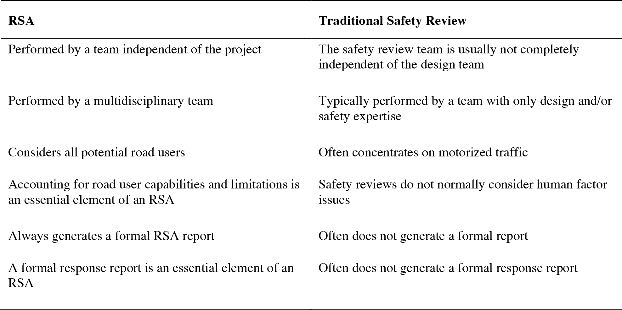
Source: Synectics Transportation Consultants Inc. et al., 2006
Long Description.
RSA: Performed by a team independent of the project. Traditional Safety Review: The safety review team is usually not completely independent of the design team. RSA: Performed by a multidisciplinary team. Traditional Safety Review: Typically performed by a team with only design and/or safety expertise. RSA: Considers all potential road users. Traditional Safety Review: Often concentrates on motorized traffic. RSA: Accounting for road user capabilities and limitations is an essential element of an RSA. Traditional Safety Review: Safety reviews do not normally consider human factor issues. RSA: Always generates a formal RSA report. Traditional Safety Review: Often does not generate a formal report. RSA: A formal response report is an essential element of an RSA. Traditional Safety Review: Often does not generate a formal response report.
Step 1 identifies the road or project to be audited, and Step 2 involves picking the RSA team.
- In Step 1, the greatest benefits to using the HFG will be obtained on RSA projects where there are some a priori reasons for believing that driver errors related to the roadway design are taking place and impacting safety performance.
- In Step 2, including someone with human factors experience or someone with experience using human factors design tools like the HFG is a good idea, especially if there are any specific concerns regarding road user behavior, capabilities, or limitations.
Steps 3, 4, and 5 of the RSA process are where the HFG will most clearly benefit RSAs, and the discussion below focuses on those activities.
- Step 3 is a pre-audit review to set the scope of the review and to share key information and documents among the RSA team. From the HFG perspective, the goal in this step is to review the relevant design information and crash history associated with the facility being audited and to create an initial list of HFG topics and materials that reflects the facilitiesʼ design features and possible safety concerns. Table 27-16 provides an overview of this activity.
- Step 4 includes a more detailed review of design drawings and project data, as well as a field review of the site. From the HFG perspective, the goal in this step is to review the relevant design information and crash history associated with the facility being audited and to create a list of HFG topics and materials that reflects the facilitiesʼ design features and safety concerns. Table 27-17 provides a sample worksheet for this activity.
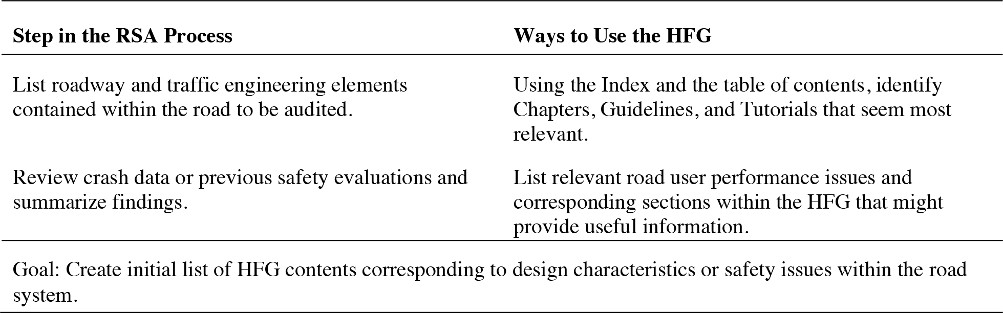
Long Description.
The steps in the RSA process listed are as follows: List roadway and traffic engineering elements contained within the road to be audited. Review crash data or previous safety evaluations and summarize findings. The ways to use the HFG are as follows: Using the Index and the table of contents, identify Chapters, Guidelines, and Tutorials that seem most relevant. List relevant road user performance issues and corresponding sections within the HFG that might provide useful information. The goal is as follows: Create initial list of HFG contents corresponding to design characteristics or safety issues within the road system.
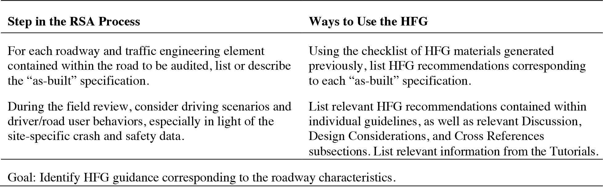
Long Description.
The steps in the RSA process listed are as follows: For each roadway and traffic engineering element contained within the road to be audited, list or describe the “as-built” specification. During the field review, consider driving scenarios and driver/road user behaviors, especially in light of the site-specific crash and safety data. The ways to use the HFG are as follows: Using the checklist of HFG materials generated previously, list HFG recommendations corresponding to each “as-built” specification. List relevant HFG recommendations contained within individual guidelines, as well as relevant Discussion, Design Issues, and Cross References subsections. List relevant information from the Tutorials. The goal is to identify HFG guidance corresponding to the roadway characteristics.
Step 5 includes conducting the audit analysis and preparing the RSA report. From the HFG perspective, the goal in this step is to assess risks related to any differences between the “as-built” specifications and the HFG recommendations and to use HFG topics and materials that address safety concerns. Table 27-18 provides a sample worksheet for this activity.
The remaining steps described by Synectics Transportation Consultants Inc. et al. (2006) are the reporting and follow-up activities for the RSA, for which the HFG is of limited relevance.
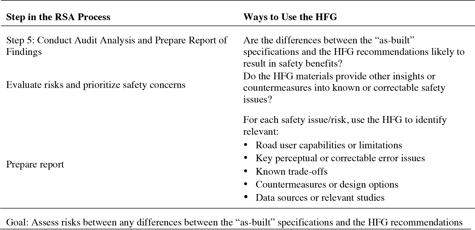
Long Description.
The steps in the RSA Process listed are as follows: Evaluate risks and priortize safety concerns. Prepare report. The ways to use the H F G are as follows: Are the differences between the “as-built” specifications and the HFG recommendations likely to result in safety benefits? Do the HFG materials provide other insights or countermeasures into known or correctable safety issues? For each safety issue/risk, use the HFG to identify relevant: Road user capabilities or limitations Key perceptual or correctable error issues Known trade-offs Countermeasures or design options Data sources or relevant studies. The goal is to assess risks between any differences between the "as-built" specifications and the HFG recommendations.


